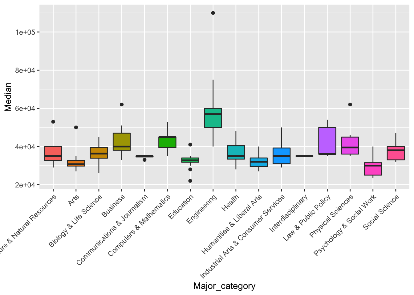
1.4 — Data Wrangling

(Answer Key)

Required Packages

First, install the following two packages with the command install.packages("tidyverse") and install.packages("gapminder") in the console below.¹ Alternatively, you will probably already get a yellow banner at the top of this file indicating you need to install the packages, and can install them by clicking Install. Don’t install any package in an R chunk in this document, since it needs to be installed into R Studio.

Then, load the package by running (clicking the green play button) the chunk below:

library("tidyverse") # my friend and yours

── Attaching packages ─────────────────────────────────────── tidyverse 1.3.1 ──

✔ ggplot2 3.3.6     ✔ purrr   0.3.4
✔ tibble  3.1.8     ✔ dplyr   1.0.9
✔ tidyr   1.2.0     ✔ stringr 1.4.0
✔ readr   2.1.2     ✔ forcats 0.5.1

── Conflicts ────────────────────────────────────────── tidyverse_conflicts() ──
✖ dplyr::filter() masks stats::filter()
✖ dplyr::lag()    masks stats::lag()

library("gapminder") # for dataset

gapminder <- gapminder # explicitly save data as a dataframe

Warm Up to dplyr with gapminder Again

Question 1

Let’s look at the data again by running the following chunk. glimpse() is a suped-up tidyverse version of str(). You can also start to see how to use the pipe operator %>%.

gapminder %>% 
  glimpse()

Rows: 1,704
Columns: 6
$ country   <fct> "Afghanistan", "Afghanistan", "Afghanistan", "Afghanistan", …
$ continent <fct> Asia, Asia, Asia, Asia, Asia, Asia, Asia, Asia, Asia, Asia, …
$ year      <int> 1952, 1957, 1962, 1967, 1972, 1977, 1982, 1987, 1992, 1997, …
$ lifeExp   <dbl> 28.801, 30.332, 31.997, 34.020, 36.088, 38.438, 39.854, 40.8…
$ pop       <int> 8425333, 9240934, 10267083, 11537966, 13079460, 14880372, 12…
$ gdpPercap <dbl> 779.4453, 820.8530, 853.1007, 836.1971, 739.9811, 786.1134, …

Question 2

Now select() only the variables year, lifeExp, and country.

gapminder %>% 
  select(year, lifeExp, country)

ABCDEFGHIJ0123456789

year <int>	lifeExp <dbl>	country <fct>
1952	28.80100	Afghanistan
1957	30.33200	Afghanistan
1962	31.99700	Afghanistan
1967	34.02000	Afghanistan
1972	36.08800	Afghanistan
1977	38.43800	Afghanistan
1982	39.85400	Afghanistan
1987	40.82200	Afghanistan
1992	41.67400	Afghanistan
1997	41.76300	Afghanistan

Next

123456

...

171

Previous

1-10 of 1,704 rows

Question 3

Now select() all variables except pop.

gapminder %>%
  select(-pop)

ABCDEFGHIJ0123456789

country <fct>	continent <fct>	year <int>	lifeExp <dbl>	gdpPercap <dbl>
Afghanistan	Asia	1952	28.80100	779.4453
Afghanistan	Asia	1957	30.33200	820.8530
Afghanistan	Asia	1962	31.99700	853.1007
Afghanistan	Asia	1967	34.02000	836.1971
Afghanistan	Asia	1972	36.08800	739.9811
Afghanistan	Asia	1977	38.43800	786.1134
Afghanistan	Asia	1982	39.85400	978.0114
Afghanistan	Asia	1987	40.82200	852.3959
Afghanistan	Asia	1992	41.67400	649.3414
Afghanistan	Asia	1997	41.76300	635.3414

Next

123456

...

171

Previous

1-10 of 1,704 rows

Question 4

rename() the variable continent to cont.

gapminder %>%
  rename(cont = continent)

ABCDEFGHIJ0123456789

country <fct>	cont <fct>	year <int>	lifeExp <dbl>	pop <int>	gdpPercap <dbl>
Afghanistan	Asia	1952	28.80100	8425333	779.4453
Afghanistan	Asia	1957	30.33200	9240934	820.8530
Afghanistan	Asia	1962	31.99700	10267083	853.1007
Afghanistan	Asia	1967	34.02000	11537966	836.1971
Afghanistan	Asia	1972	36.08800	13079460	739.9811
Afghanistan	Asia	1977	38.43800	14880372	786.1134
Afghanistan	Asia	1982	39.85400	12881816	978.0114
Afghanistan	Asia	1987	40.82200	13867957	852.3959
Afghanistan	Asia	1992	41.67400	16317921	649.3414
Afghanistan	Asia	1997	41.76300	22227415	635.3414

Next

123456

...

171

Previous

1-10 of 1,704 rows

Question 5

arrange() the data by year.

gapminder %>%
  arrange(year)

ABCDEFGHIJ0123456789

country <fct>	continent <fct>	year <int>	lifeExp <dbl>
Afghanistan	Asia	1952	28.80100
Albania	Europe	1952	55.23000
Algeria	Africa	1952	43.07700
Angola	Africa	1952	30.01500
Argentina	Americas	1952	62.48500
Australia	Oceania	1952	69.12000
Austria	Europe	1952	66.80000
Bahrain	Asia	1952	50.93900
Bangladesh	Asia	1952	37.48400
Belgium	Europe	1952	68.00000

Next

123456

...

171

Previous

1-10 of 1,704 rows | 1-4 of 6 columns

Question 6

Now arrange() by year, but in descending order.

gapminder %>%
  arrange(desc(year))

ABCDEFGHIJ0123456789

country <fct>	continent <fct>	year <int>	lifeExp <dbl>
Afghanistan	Asia	2007	43.82800
Albania	Europe	2007	76.42300
Algeria	Africa	2007	72.30100
Angola	Africa	2007	42.73100
Argentina	Americas	2007	75.32000
Australia	Oceania	2007	81.23500
Austria	Europe	2007	79.82900
Bahrain	Asia	2007	75.63500
Bangladesh	Asia	2007	64.06200
Belgium	Europe	2007	79.44100

Next

123456

...

171

Previous

1-10 of 1,704 rows | 1-4 of 6 columns

Question 7

Now arrange() by year, then by lifeExp

gapminder %>%
  arrange(year, lifeExp)

ABCDEFGHIJ0123456789

country <fct>	continent <fct>	year <int>	lifeExp <dbl>
Afghanistan	Asia	1952	28.80100
Gambia	Africa	1952	30.00000
Angola	Africa	1952	30.01500
Sierra Leone	Africa	1952	30.33100
Mozambique	Africa	1952	31.28600
Burkina Faso	Africa	1952	31.97500
Guinea-Bissau	Africa	1952	32.50000
Yemen, Rep.	Asia	1952	32.54800
Somalia	Africa	1952	32.97800
Guinea	Africa	1952	33.60900

Next

123456

...

171

Previous

1-10 of 1,704 rows | 1-4 of 6 columns

Question 8

Let’s try subsetting some rows. filter() observations with pop greater than 1 billion (9 zeros).

gapminder %>%
  filter(pop > 1000000000)

ABCDEFGHIJ0123456789

country <fct>	continent <fct>	year <int>	lifeExp <dbl>	pop <int>	gdpPercap <dbl>
China	Asia	1982	65.525	1000281000	962.4214
China	Asia	1987	67.274	1084035000	1378.9040
China	Asia	1992	68.690	1164970000	1655.7842
China	Asia	1997	70.426	1230075000	2289.2341
China	Asia	2002	72.028	1280400000	3119.2809
China	Asia	2007	72.961	1318683096	4959.1149
India	Asia	2002	62.879	1034172547	1746.7695
India	Asia	2007	64.698	1110396331	2452.2104

8 rows

Question 9

Redo the same command from question 8, but of that subset of data, only look at India.

gapminder %>%
  filter(pop > 1000000000,
         country == "India")

ABCDEFGHIJ0123456789

country <fct>	continent <fct>	year <int>	lifeExp <dbl>	pop <int>	gdpPercap <dbl>
India	Asia	2002	62.879	1034172547	1746.769
India	Asia	2007	64.698	1110396331	2452.210

2 rows

Question 10

Let’s pipe a bunch of commands together. select() your data to look only at year, gdpPercap, and country in the year 1997, for countries that have a gdpPercap greater than 20,000, and arrange() them alphabetically.

gapminder %>%
  select(year, gdpPercap, country) %>%
  filter(year == 1997,
         gdpPercap > 20000) %>%
  arrange(country)

ABCDEFGHIJ0123456789

year <int>	gdpPercap <dbl>	country <fct>
1997	26997.94	Australia
1997	29095.92	Austria
1997	20292.02	Bahrain
1997	27561.20	Belgium
1997	28954.93	Canada
1997	29804.35	Denmark
1997	23723.95	Finland
1997	25889.78	France
1997	27788.88	Germany
1997	28377.63	Hong Kong, China

Next

123

Previous

1-10 of 27 rows

Question 11

Make a new variable with mutate() called GDP, which is equal to gdpPercap * pop.

gapminder %>%
  mutate(GDP = gdpPercap * pop)

ABCDEFGHIJ0123456789

country <fct>	continent <fct>	year <int>	lifeExp <dbl>	pop <int>	gdpPercap <dbl>
Afghanistan	Asia	1952	28.80100	8425333	779.4453
Afghanistan	Asia	1957	30.33200	9240934	820.8530
Afghanistan	Asia	1962	31.99700	10267083	853.1007
Afghanistan	Asia	1967	34.02000	11537966	836.1971
Afghanistan	Asia	1972	36.08800	13079460	739.9811
Afghanistan	Asia	1977	38.43800	14880372	786.1134
Afghanistan	Asia	1982	39.85400	12881816	978.0114
Afghanistan	Asia	1987	40.82200	13867957	852.3959
Afghanistan	Asia	1992	41.67400	16317921	649.3414
Afghanistan	Asia	1997	41.76300	22227415	635.3414

Next

123456

...

171

Previous

1-10 of 1,704 rows | 1-6 of 7 columns

Question 12

Make a new variable that is pop in millions.

gapminder %>%
  mutate(pop_mil = pop / 1000000)

ABCDEFGHIJ0123456789

country <fct>	continent <fct>	year <int>	lifeExp <dbl>	pop <int>	gdpPercap <dbl>
Afghanistan	Asia	1952	28.80100	8425333	779.4453
Afghanistan	Asia	1957	30.33200	9240934	820.8530
Afghanistan	Asia	1962	31.99700	10267083	853.1007
Afghanistan	Asia	1967	34.02000	11537966	836.1971
Afghanistan	Asia	1972	36.08800	13079460	739.9811
Afghanistan	Asia	1977	38.43800	14880372	786.1134
Afghanistan	Asia	1982	39.85400	12881816	978.0114
Afghanistan	Asia	1987	40.82200	13867957	852.3959
Afghanistan	Asia	1992	41.67400	16317921	649.3414
Afghanistan	Asia	1997	41.76300	22227415	635.3414

Next

123456

...

171

Previous

1-10 of 1,704 rows | 1-6 of 7 columns

Question 13

Use the summarize() command to get the overall average GDP per capita in the data.

gapminder %>%
  summarize(avg_gdppc = mean(gdpPercap))

ABCDEFGHIJ0123456789

avg_gdppc <dbl>
7215.327

1 row

Question 14

Use summarize() to get the number of observations, the mean, median, minimum, maximum, and standard deviation of GDP per capita.

gapminder %>%
  summarize(n(),
            mean_GDP = mean(gdpPercap),
            median_GDP = median(gdpPercap),
            min_GDP = min(gdpPercap),
            max_GDP = max(gdpPercap),
            sd_GDP = sd(gdpPercap))

ABCDEFGHIJ0123456789

n() <int>	mean_GDP <dbl>	median_GDP <dbl>	min_GDP <dbl>	max_GDP <dbl>	sd_GDP <dbl>
1704	7215.327	3531.847	241.1659	113523.1	9857.455

1 row

Question 15

The code below gets the average GDP per capita by continent. Run it to see the results.

gapminder %>%
  group_by(continent) %>%
  summarize(avg_gdppc = mean(gdpPercap))

ABCDEFGHIJ0123456789

continent <fct>	avg_gdppc <dbl>
Africa	2193.755
Americas	7136.110
Asia	7902.150
Europe	14469.476
Oceania	18621.609

5 rows

Now, modify it to show the average GDP per capita by year (i.e. over time).

gapminder %>%
  group_by(year) %>%
  summarize(avg_gdppc = mean(gdpPercap))

ABCDEFGHIJ0123456789

year <int>	avg_gdppc <dbl>
1952	3725.276
1957	4299.408
1962	4725.812
1967	5483.653
1972	6770.083
1977	7313.166
1982	7518.902
1987	7900.920
1992	8158.609
1997	9090.175

Next

12

Previous

1-10 of 12 rows

Question 16

Get the average GDP per capita by year and by continent with group_by() and summarize(). Then save this as an object. Next, make a line graph with ggplot() (automatically loaded with tidyverse!) using this object as the source for your data layer. Be sure to map color = continent in the aes layer! This should plot GDP per capita over time by continent.

gdp_grouped <- gapminder %>%
  group_by(year, continent) %>%
  summarize(Average_GDP = mean(gdpPercap))

`summarise()` has grouped output by 'year'. You can override using the
`.groups` argument.

ggplot(data = gdp_grouped) +
  aes(x = year,
      y = Average_GDP,
      color = continent) +
  geom_line()

Question 17

Copy your code from question 16 and redo this all in one step: rather than saving your subsetted data as an object, pipe it directly into ggplot’s data layer!

gapminder %>%
  group_by(year, continent) %>%
  summarize(Average_GDP = mean(gdpPercap)) %>%
ggplot(data = .) +
  aes(x = year,
      y = Average_GDP,
      color = continent) +
  geom_line()

`summarise()` has grouped output by 'year'. You can override using the
`.groups` argument.

An Example Data: Majors

Now let’s step it up to work with some data “in the wild” to answer some research questions. This will have you combine your dplyr skills and add some new things such as importing with readr.

Let’s look at fivethirtyeight’s article ” The Economic Guide To Picking A College Major ”. fivethirtyeight is great about making the data behind their articles public, we can download all of their data here. Search for college majors and click download (the blue arrow button).² We will look at the recent-grads.csv file.

The description in the readme file for the data is as follows:

Header	Description
Rank	Rank by median earnings
Major_code	Major code, FO1DP in ACS PUMS
Major	Major description
Major_category	Category of major from Carnevale et al
Total	Total number of people with major
Sample_size	Sample size (unweighted) of full-time, year-round ONLY (used for earnings)
Men	Male graduates
Women	Female graduates
ShareWomen	Women as share of total
Employed	Number employed (ESR == 1 or 2)
Full_time	Employed 35 hours or more
Part_time	Employed less than 35 hours
Full_time_year_round	Employed at least 50 weeks (WKW == 1) and at least 35 hours (WKHP >= 35)
Unemployed	Number unemployed (ESR == 3)
Unemployment_rate	Unemployed / (Unemployed + Employed)
Median	Median earnings of full-time, year-round workers
P25th	25th percentile of earnigns
P75th	75th percentile of earnings
College_jobs	Number with job requiring a college degree
Non_college_jobs	Number with job not requiring a college degree
Low_wage_jobs	Number in low-wage service jobs

Question 18

Import the data with read_csv() and assign it to an object (a tibble) called majors (or whatever you want to call it).

One way to avoid problems is to move this to the same file as R’s working directory, which again you can determine with getwd(). If you are doing this in R Studio Cloud, use the Upload button to add the file to the working directory (once you’ve downloaded it from the internet!). If you are doing this on your computer, move the downloaded file on your computer to wherever your R Project folder for this project is.

majors <- read_csv("../data/recent-grads.csv") # note my location on my computer is different than yours!

Rows: 173 Columns: 21
── Column specification ────────────────────────────────────────────────────────
Delimiter: ","
chr  (2): Major, Major_category
dbl (19): Rank, Major_code, Total, Men, Women, ShareWomen, Sample_size, Empl...

ℹ Use `spec()` to retrieve the full column specification for this data.
ℹ Specify the column types or set `show_col_types = FALSE` to quiet this message.

Once it’s loaded, get a look at the data with glimpse:

majors %>% # or whatever you named your tibble with the data
  glimpse()

Rows: 173
Columns: 21
$ Rank                 <dbl> 1, 2, 3, 4, 5, 6, 7, 8, 9, 10, 11, 12, 13, 14, 15…
$ Major_code           <dbl> 2419, 2416, 2415, 2417, 2405, 2418, 6202, 5001, 2…
$ Major                <chr> "PETROLEUM ENGINEERING", "MINING AND MINERAL ENGI…
$ Total                <dbl> 2339, 756, 856, 1258, 32260, 2573, 3777, 1792, 91…
$ Men                  <dbl> 2057, 679, 725, 1123, 21239, 2200, 2110, 832, 803…
$ Women                <dbl> 282, 77, 131, 135, 11021, 373, 1667, 960, 10907, …
$ Major_category       <chr> "Engineering", "Engineering", "Engineering", "Eng…
$ ShareWomen           <dbl> 0.1205643, 0.1018519, 0.1530374, 0.1073132, 0.341…
$ Sample_size          <dbl> 36, 7, 3, 16, 289, 17, 51, 10, 1029, 631, 399, 14…
$ Employed             <dbl> 1976, 640, 648, 758, 25694, 1857, 2912, 1526, 764…
$ Full_time            <dbl> 1849, 556, 558, 1069, 23170, 2038, 2924, 1085, 71…
$ Part_time            <dbl> 270, 170, 133, 150, 5180, 264, 296, 553, 13101, 1…
$ Full_time_year_round <dbl> 1207, 388, 340, 692, 16697, 1449, 2482, 827, 5463…
$ Unemployed           <dbl> 37, 85, 16, 40, 1672, 400, 308, 33, 4650, 3895, 2…
$ Unemployment_rate    <dbl> 0.018380527, 0.117241379, 0.024096386, 0.05012531…
$ Median               <dbl> 110000, 75000, 73000, 70000, 65000, 65000, 62000,…
$ P25th                <dbl> 95000, 55000, 50000, 43000, 50000, 50000, 53000, …
$ P75th                <dbl> 125000, 90000, 105000, 80000, 75000, 102000, 7200…
$ College_jobs         <dbl> 1534, 350, 456, 529, 18314, 1142, 1768, 972, 5284…
$ Non_college_jobs     <dbl> 364, 257, 176, 102, 4440, 657, 314, 500, 16384, 1…
$ Low_wage_jobs        <dbl> 193, 50, 0, 0, 972, 244, 259, 220, 3253, 3170, 98…

Question 19

What are all the unique values of Major? How many are there?

# distinct values of major
majors %>%
  distinct(Major)

ABCDEFGHIJ0123456789

Major <chr>
PETROLEUM ENGINEERING
MINING AND MINERAL ENGINEERING
METALLURGICAL ENGINEERING
NAVAL ARCHITECTURE AND MARINE ENGINEERING
CHEMICAL ENGINEERING
NUCLEAR ENGINEERING
ACTUARIAL SCIENCE
ASTRONOMY AND ASTROPHYSICS
MECHANICAL ENGINEERING
ELECTRICAL ENGINEERING

Next

123456

...

18

Previous

1-10 of 173 rows

# count number of distinct values
majors %>%
  summarize(n_distinct(Major))

ABCDEFGHIJ0123456789

n_distinct(Major) <int>
173

1 row

Question 20

Which major has the lowest unemployment rate?

majors %>%
  arrange(Unemployment_rate) %>%
  select(Major, Unemployment_rate)

ABCDEFGHIJ0123456789

Major <chr>
MATHEMATICS AND COMPUTER SCIENCE
MILITARY TECHNOLOGIES
BOTANY
SOIL SCIENCE
EDUCATIONAL ADMINISTRATION AND SUPERVISION
ENGINEERING MECHANICS PHYSICS AND SCIENCE
COURT REPORTING
MATHEMATICS TEACHER EDUCATION
PETROLEUM ENGINEERING
GENERAL AGRICULTURE

Next

123456

...

18

Previous

1-10 of 173 rows | 1-1 of 2 columns

Question 21

What are the top three majors that have the highest percentage of women?

majors %>%
  arrange(desc(ShareWomen)) %>%
  select(Major, ShareWomen) %>%
  slice(1:3) # head(n=3) also works

ABCDEFGHIJ0123456789

Major <chr>	ShareWomen <dbl>
EARLY CHILDHOOD EDUCATION	0.9689537
COMMUNICATION DISORDERS SCIENCES AND SERVICES	0.9679981
MEDICAL ASSISTING SERVICES	0.9278072

3 rows

Question 22

Make a boxplot of Median wage by Major_Category.

ggplot(data = majors)+
  aes(x = Major_category,
      y = Median,
      fill = Major_category)+
  geom_boxplot()+
  theme(axis.text.x=element_text(angle=45, hjust=1), legend.position = "")

Question 23

Is there a systematic difference between STEM majors and non-STEM majors? First, define

stem_categories <- c("Biology & Life Science",
                     "Computers & Mathematics",
                     "Engineering",
                     "Physical Sciences")

Next, make a variable stem, for whether or not a Major_category is "stem" or "not stem".

majors <- majors %>%
  mutate(stem = ifelse(Major_category %in% stem_categories,
                       yes = "stem",
                       no = "not_stem")) %>%
  select(stem, everything()) # just so we can see it up front to verify

# instead of ifelse(), you could use case_when:

majors %>%
  mutate(stem = case_when(Major_category %in% stem_categories ~ "stem",
                          TRUE ~ "not_stem")) # remaining case if not for stem 

ABCDEFGHIJ0123456789

stem <chr>	Rank <dbl>	Major_code <dbl>
stem	1	2419
stem	2	2416
stem	3	2415
stem	4	2417
stem	5	2405
stem	6	2418
not_stem	7	6202
stem	8	5001
stem	9	2414
stem	10	2408

Next

123456

...

18

Previous

1-10 of 173 rows | 1-3 of 22 columns

Finally, summarize() Median for stem and not stem groups.

majors %>%
  group_by(stem) %>%
  summarize(mean(Median))

ABCDEFGHIJ0123456789

stem <chr>	mean(Median) <dbl>
not_stem	35624.77
stem	47860.94

2 rows

Footnotes

1. Note that you can install multiple packages at the same time by combining the package names into a vector, like so: install.packages(c("tidyverse", "gapminder")).

2. This will download a .zip file that contains many spreadsheets. Unzip it with a program that unzips files (such as WinZip, 7-zip, the Unarchiver, etc).