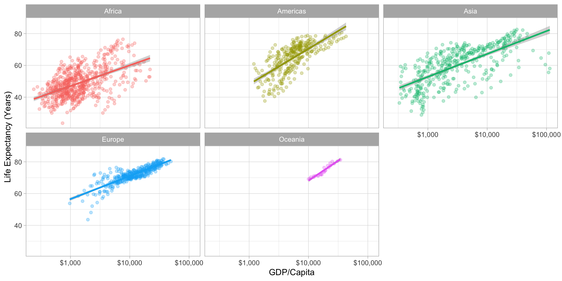
ggplot(data = gapminder,
       aes(x = gdpPercap,
           y = lifeExp,
           color = continent))+
  geom_point(alpha=0.3)+
  geom_smooth(method = "lm")+
    scale_x_log10(breaks=c(1000,10000, 100000),
                  label=scales::dollar)+
    labs(x = "GDP/Capita",
         y = "Life Expectancy (Years)")+
  facet_wrap(~continent)+
  guides(color = F)+
theme_light()R
Free and open source
A very large community
- Written by statisticians for statistics
- Most packages are written for
Rfirst
Can handle virtually any data format
Makes replication easy
Can integrate into documents (with
R markdown)R is a language so it can do everything
- A good stepping stone to learning other languages like Python

Excel (or Stata) Can’t Do This
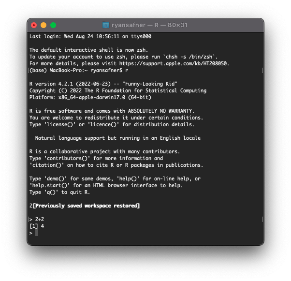
R and R Studio
R is the programming language that executes commands
Could run this from your computer’s shell
- On Windows: Command prompt
- On Mac/Linux: Terminal
R and R Studio
- R Studio1 is an integrated development environment (IDE) that makes your coding life a lot easier
- Write code in scripts
- Execute individual commands & scripts
- Auto-complete, highlight syntax
- View data, objects, and plots
- Get help and documentation on commands and functions
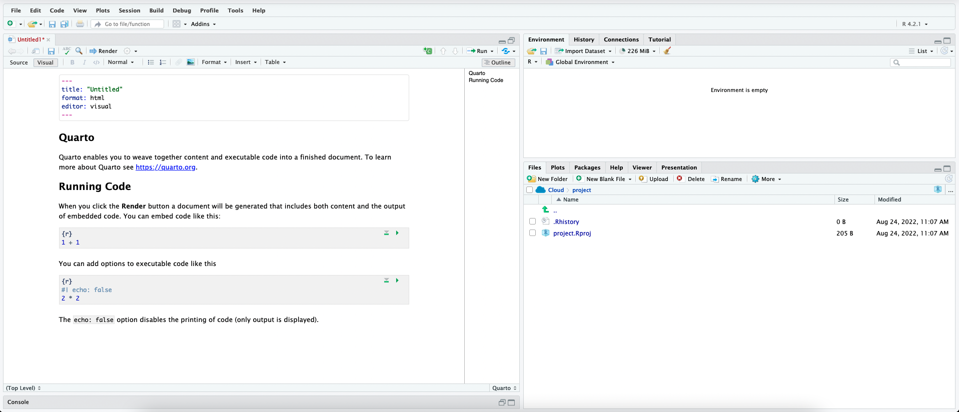
- Integrate code into documents with
Quarto
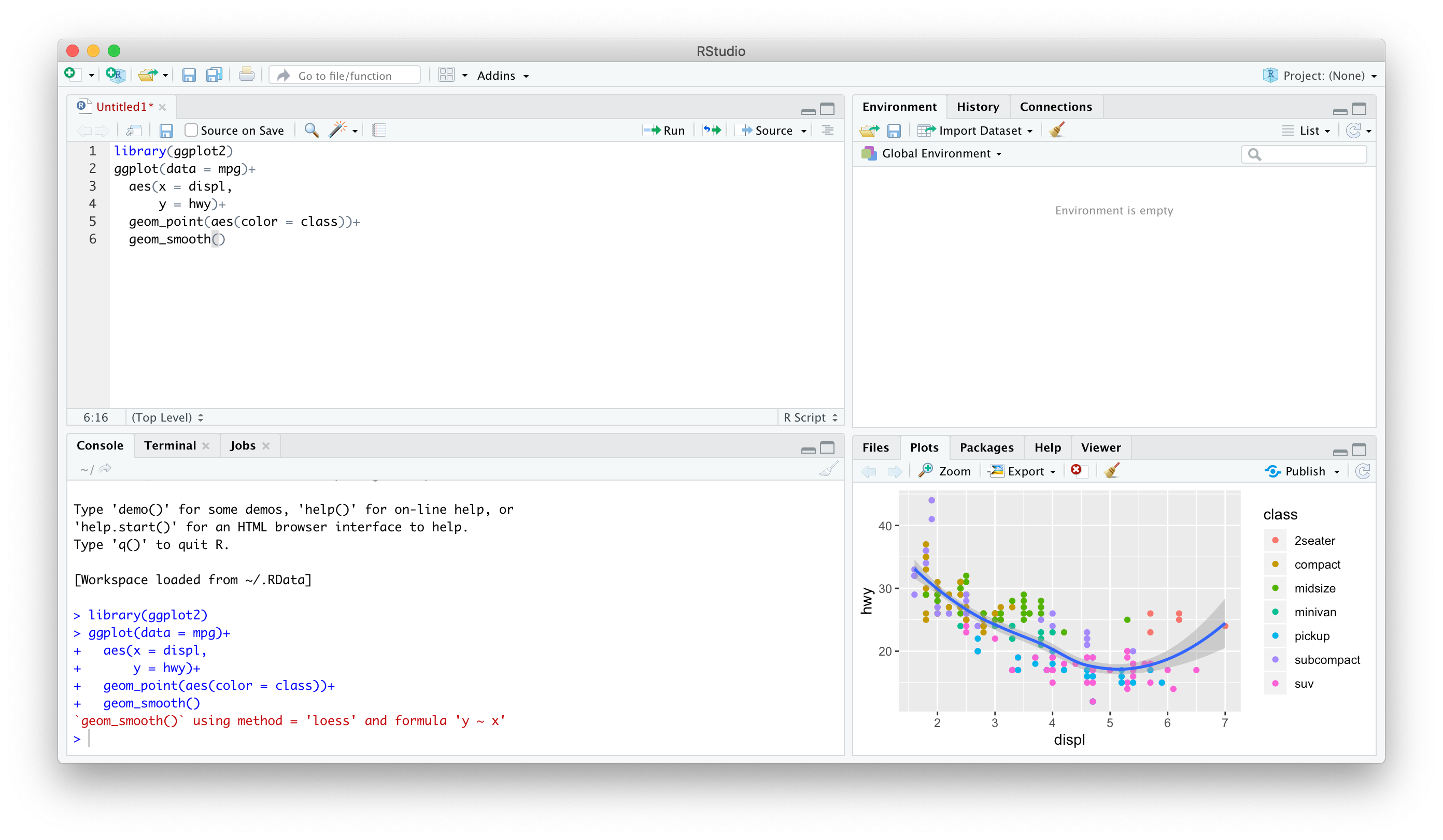
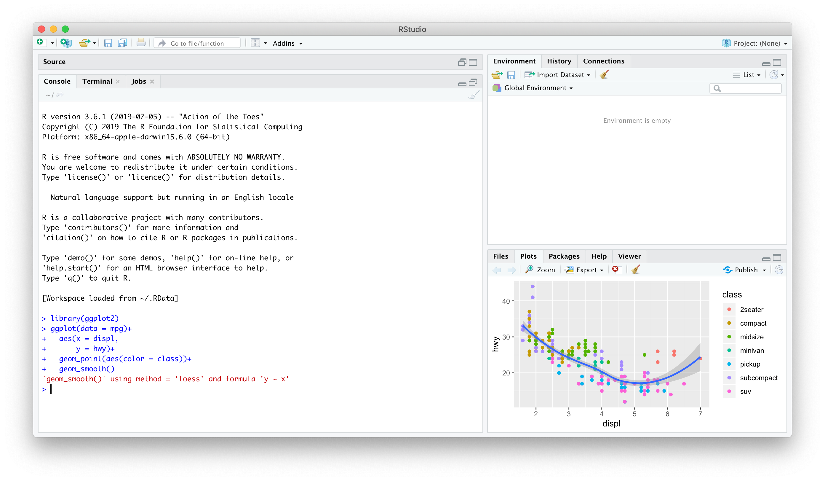
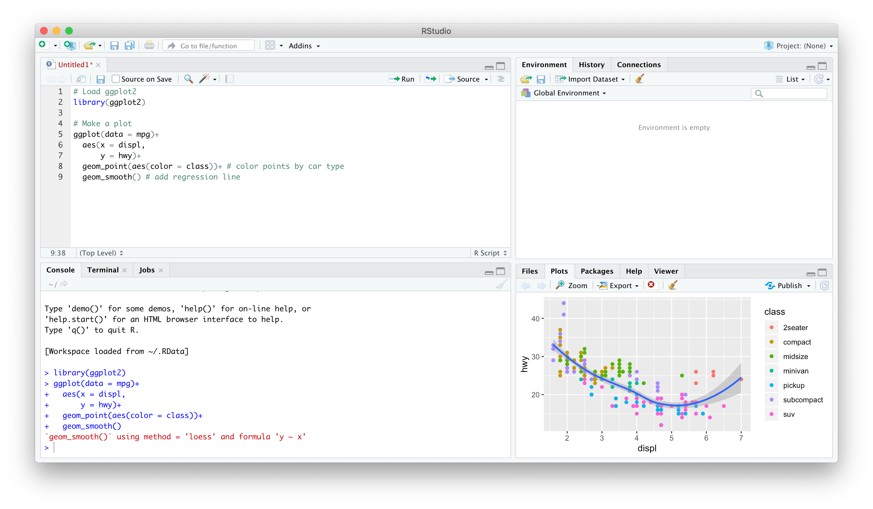
R Studio — Four Panes
Ways to Use R Studio: Using the Console
Type individual commands into the console pane (bottom left)
Great for testing individual commands to see what happens
Not saved! Not reproducible! Not recommended!
Ways to Use R Studio: Writing a .R Script
Source pane is a text-editor
Make
.Rfiles: all input commands in a single scriptComment with
#Can run any or all of script at once
Can save, reproduce, and send to others!
Ways to Use R Studio: Quarto Documents
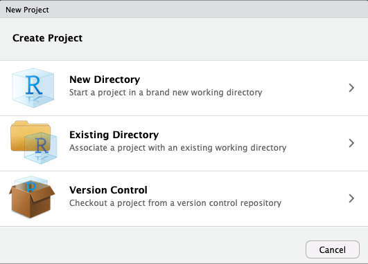
Avoid this Hassle with R Projects
- A
R Projectis a way of systematically organizing yourRhistory, working directory, and related files in a single, self-contained directory - Can easily be sent to others who can reproduce your work easily
- Connects well with version control software like GitHub
- Can open multiple projects in multiple windows
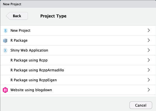
Avoid this Hassle with R Projects
In almost all cases, you simply want a
New ProjectFor more advanced uses, your project can be an
R Packageor aShiny Web ApplicationIf you have other packages that create templates installed (as I do, in the previous image), they will also show up as options
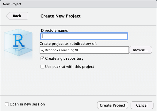
Avoid this Hassle with R Projects
Enter a name for the project in the top field
- Also creates a folder on your computer with the name you enter into the field
Choose the location of the folder on your computer
Depending on if you have other packages or utilities installed (such as
git, see below!), there may be additional options, do not check them unless you know what you are doingBottom left checkbox allows you to open a new instance (window) of
Rjust for this project (and keep existing windows open)
…and Sucking

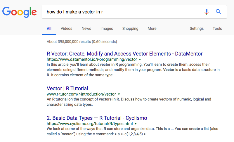
Say Hello To My Little Friend
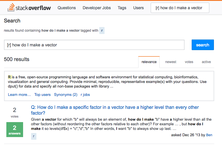
Say Hello to My Better Friend
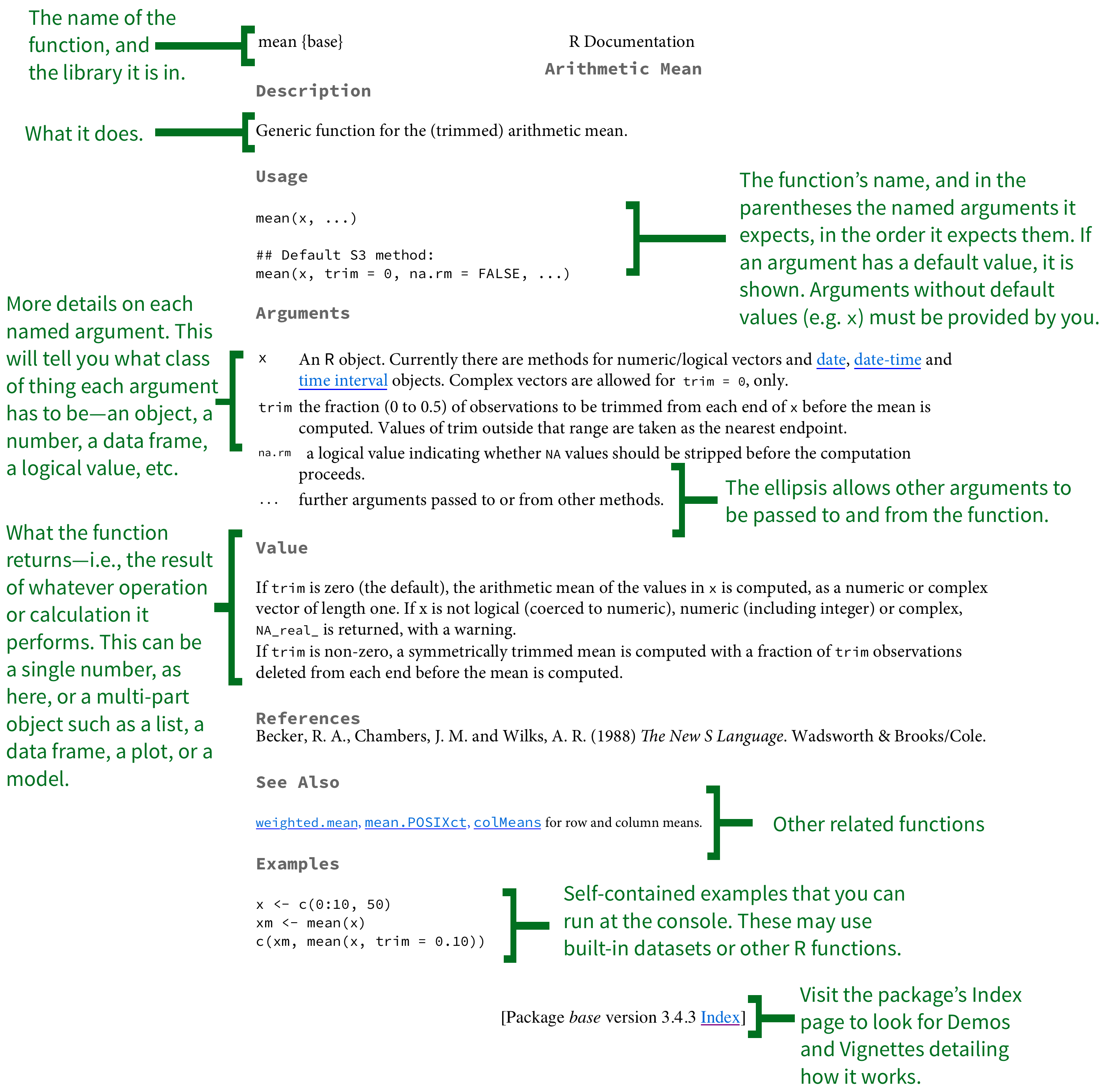
R Is Helpful Too!
- Type
help(function_name)or?(function_name)to get documentation on a function
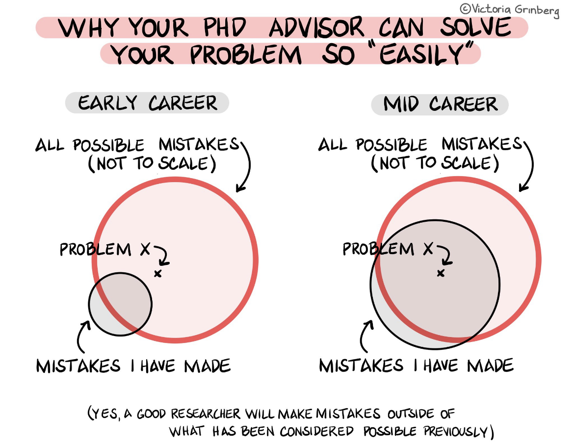
I’ve Failed More Times Than You
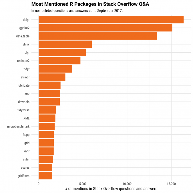
Packages and Libraries
- Since R is open source, users contribute packages
- Really it’s just users writing custom functions and saving them for others to use
- Load packages with
library()1- e.g.
library("ggplot2")
- e.g.
- If you don’t have a package, you must first
install.packages()2- e.g.
install.packages("ggplot2")
- e.g.
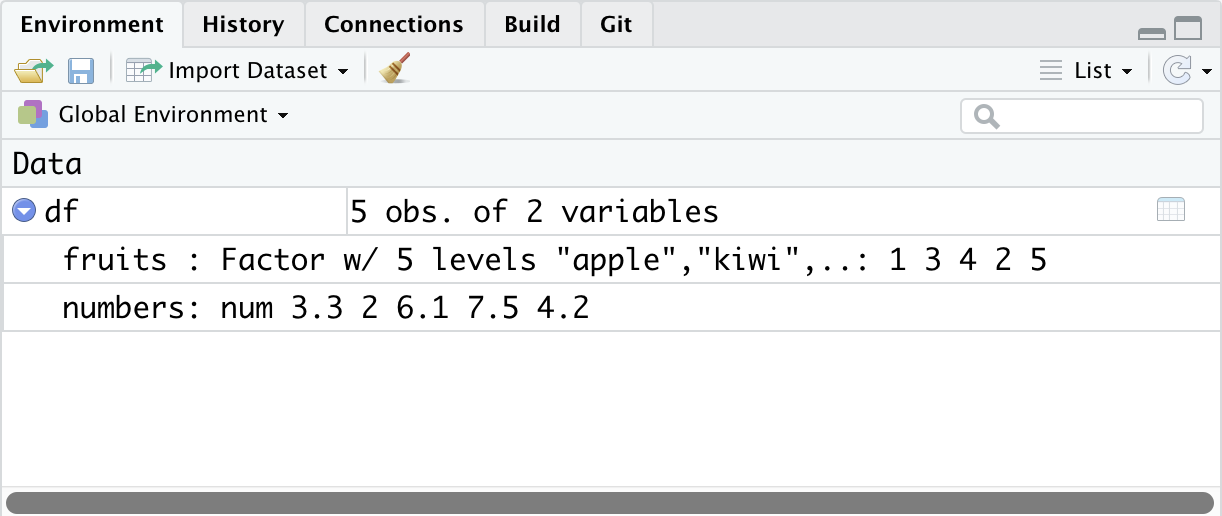
More on Dataframes IV
- Note, once you save an object, it shows up in the Environment Pane in the upper right window
- Click the blue arrow button in front of the object for some more information
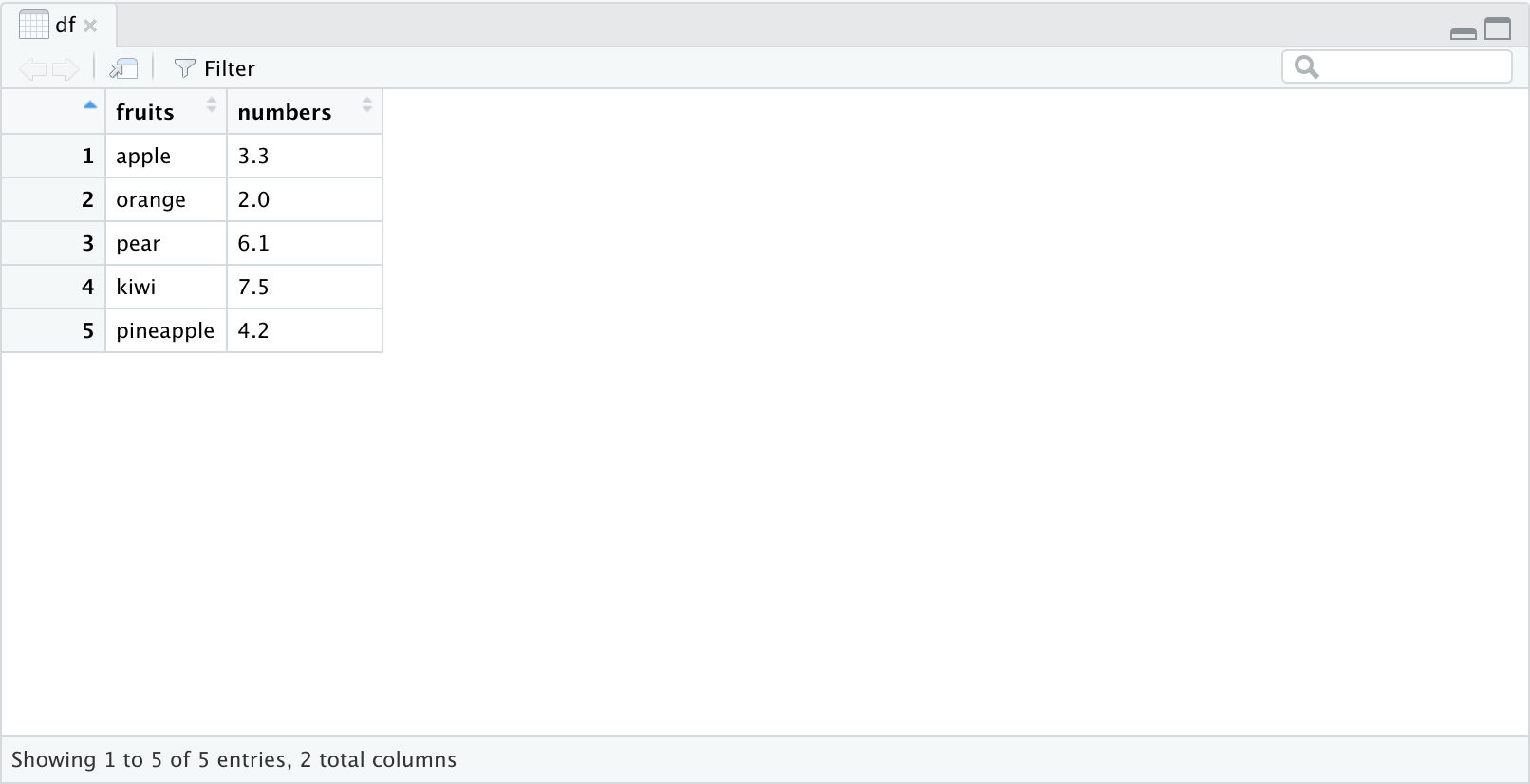
More on Dataframes V
data.frameobjects can be viewed in their own panel by clicking on the name of the object in the environment pane- Note you cannot edit anything in this pane, it is for viewing only
Some Common Errors
- If you make a coding error (e.g. forget to close a parenthesis), R might show a
+sign waiting for you to finish the command
- Either finish the command– e.g. add
)–or hitEscto cancel
