Data Wrangling
- Most data analysis is taming chaos into order
- Data strewn from multiple sources 😨
- Missing data (“
NA”) 😡 - Data not in a readable form 🤢

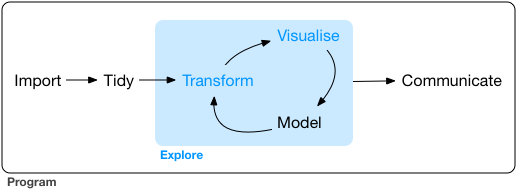
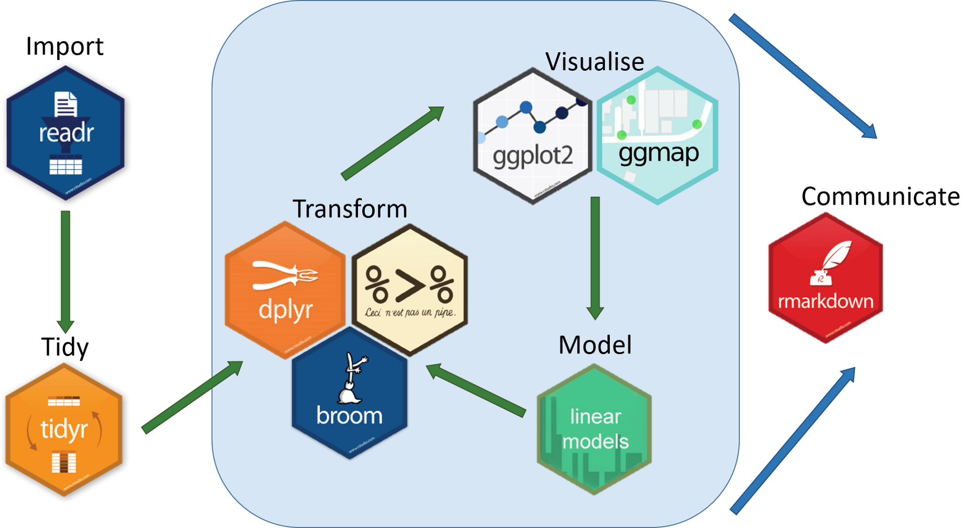
Workflow of a Data Scientist I
- Import raw data from out there in the world
- Tidy it into a form that you can use
- Explore the data (do these 3 repetitively!)
- Transform
- Visualize
- Model
- Communicate results to target audience
Ideally, you’d want to be able to do all of this in one program
Workflow of a Data Scientist II
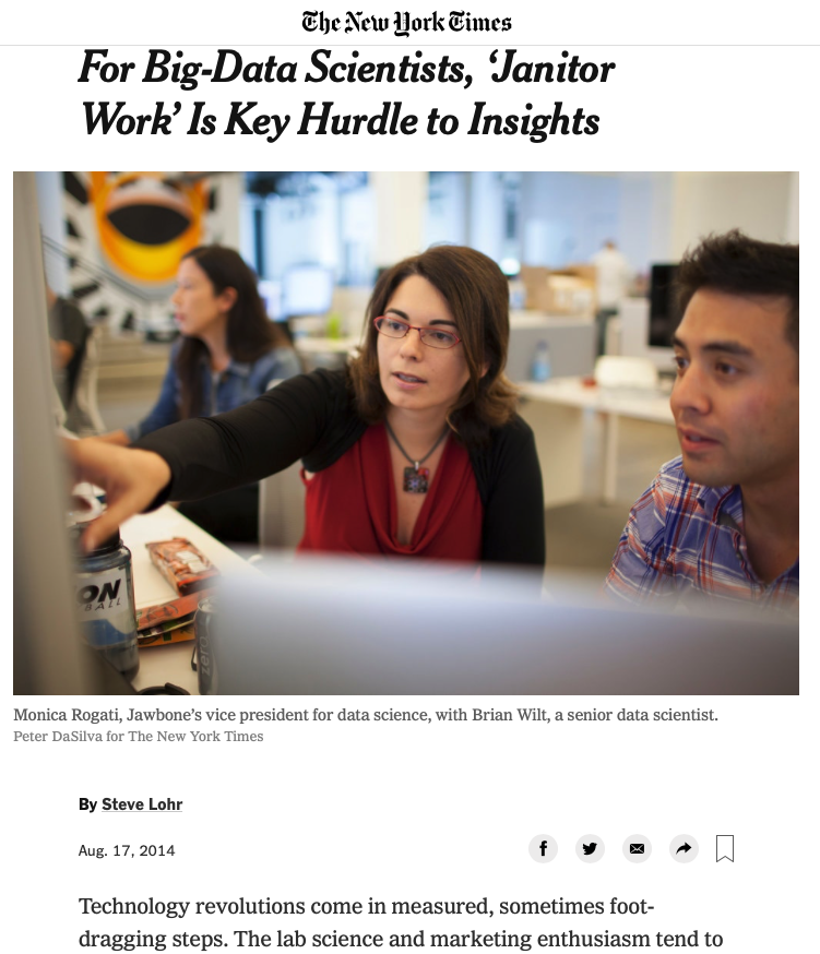
“Yet far too much handcrafted work - what data scientists call”data wrangling,” “data munging,” and “data janitor work” - is still required. Data scientists, according to interviews and expert estimates, spend from 50 to 80 percent of their time mired in this more mundane labor of collecting and preparing unruly digital data, before it can be explored for useful nuggets.”
Source: New York Times
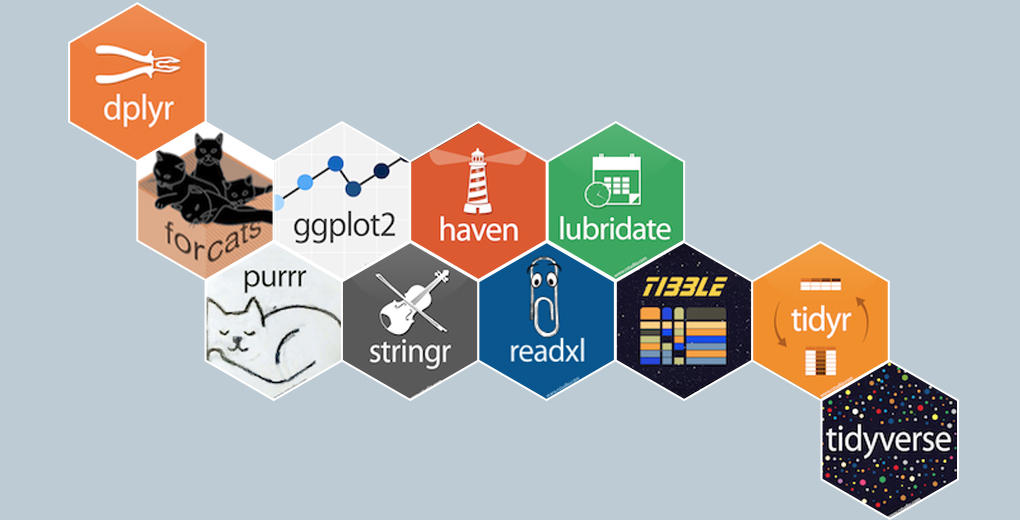
The tidyverse I
“The tidyverse is an opinionated collection of R packages designed for data science. All packages share an underlying design philosophy, grammar, and data structures.
- Allows you to do all of those things with one (set of) package(s)!
- Learn more at tidyverse.org
The tidyverse II
Your Workflow in the tidyverse:
Tibbles
A
tibble(ortbl_df) is a friendlierdata.frameFundamental grammar of tidyverse:
- start with a tibble
- run a function on it
- output a new tibble
Loading
tidyverseautomatically converts alldata.framestotibbles
Tibbles: Making a Tibble
- Create a
tibblefrom adata.framewithas_tibble()
# A tibble: 53,940 × 10
   carat cut       color clarity depth table price     x     y     z
   <dbl> <ord>     <ord> <ord>   <dbl> <dbl> <int> <dbl> <dbl> <dbl>
 1  0.23 Ideal     E     SI2      61.5    55   326  3.95  3.98  2.43
 2  0.21 Premium   E     SI1      59.8    61   326  3.89  3.84  2.31
 3  0.23 Good      E     VS1      56.9    65   327  4.05  4.07  2.31
 4  0.29 Premium   I     VS2      62.4    58   334  4.2   4.23  2.63
 5  0.31 Good      J     SI2      63.3    58   335  4.34  4.35  2.75
 6  0.24 Very Good J     VVS2     62.8    57   336  3.94  3.96  2.48
 7  0.24 Very Good I     VVS1     62.3    57   336  3.95  3.98  2.47
 8  0.26 Very Good H     SI1      61.9    55   337  4.07  4.11  2.53
 9  0.22 Fair      E     VS2      65.1    61   337  3.87  3.78  2.49
10  0.23 Very Good H     VS1      59.4    61   338  4     4.05  2.39
# … with 53,930 more rows
Tibbles: Making a Tibble (from Scratch)
- Create a
tibblefrom scratch withtibble(), works likedata.frame()
Tibbles: Making a Tibble (from Scratch)
- Create a
tibblerow by row withtribble()
Piping Code
The
magrittrpackage allows use of the “pipe” operator (%>%)1%>%“pipes” the output of the left of the pipe into the (1st) argument of the rightRunning a function
fon objectxasf(x)becomesx %>% fin pipeable form- i.e. “take
xand then run functionfon it”
- i.e. “take
Importing Data I

Load common spreadsheet files (
.csv,.tsv) with simple commands:read_*(path/to/my_data.*)- where
*can be.csvor.tsv
- where
Can also export your data from R into a common spreadsheet file with:
write_*(my_df, path = path/to/file_name.*)- where
my_dfis the name of yourtibble, andfile_nameis the name of the file you want to save as
- where
Often this is enough, but much more customization possible
Read more on the tidyverse website and the Readr Cheatsheet
Importing Data II


- For other data types from software programs like Excel, STATA, SAS, and SPSS:
readxlhas equivalent commands for Excel data types:read_*("path/to/my/data.*")write_*(my_dataframe, path=path/to/file_name.*)- where
*can be.xlsor.xlsx
havenhas equivalent commands for other data types:read_*("path/to/my_data.dta")for STATA.dtafileswrite_*(my_dataframe, path=path/to/file_name.*)- where
*can be.dta(STATA),.sav(SPSS),.sas7bdat(SAS)
Data Import Cheat Sheet

Tidying (Pivoting/Reshaping) Data
Tidy Data
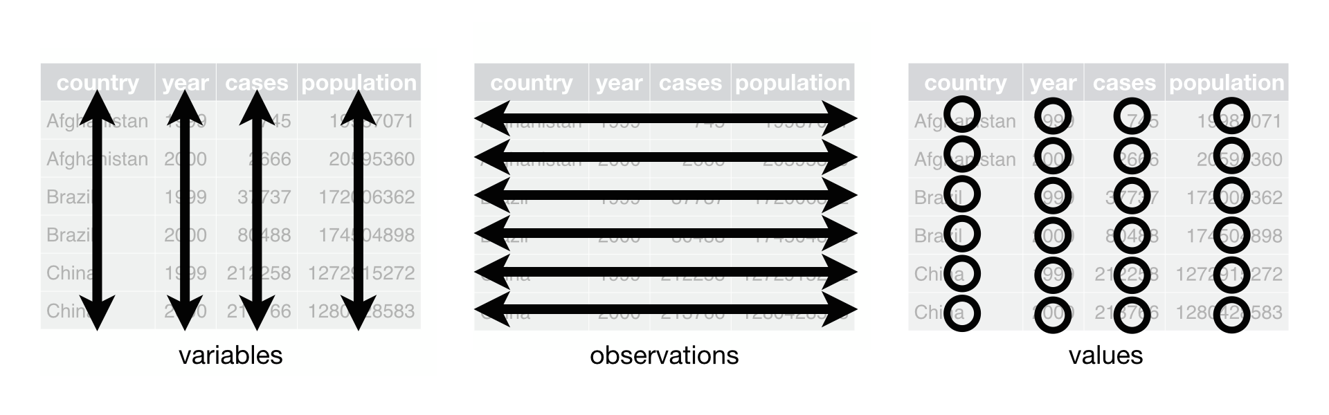
- “tidy” data are (an opinionated view of) data where
- Each variable is in a column
- Each observation is a row
- Each observational unit forms a table (or “every value is its own cell.”)
- This is the namesake of the
tidyverse: all associated packages and functions require tidy data- Spend less time fighting your tools and more time on analysis!
Tidy vs. Untidy Data
- “Tidy” data \(\neq\) clean, perfect data
“Happy families are all alike; every unhappy family is unhappy in its own way.” - Leo Tolstoy
“Tidy datasets are all alike, but every messy dataset is messy in its own way.” - Hadley Wickham
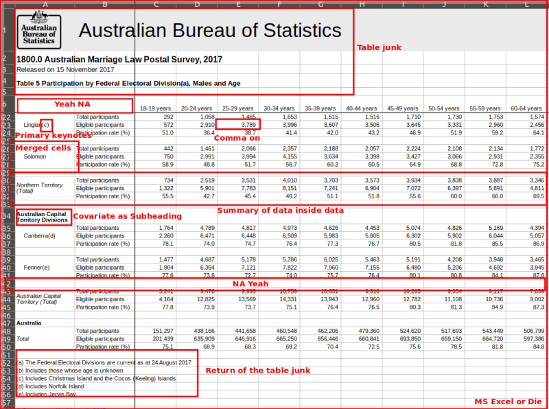
Examples of Untidy Data
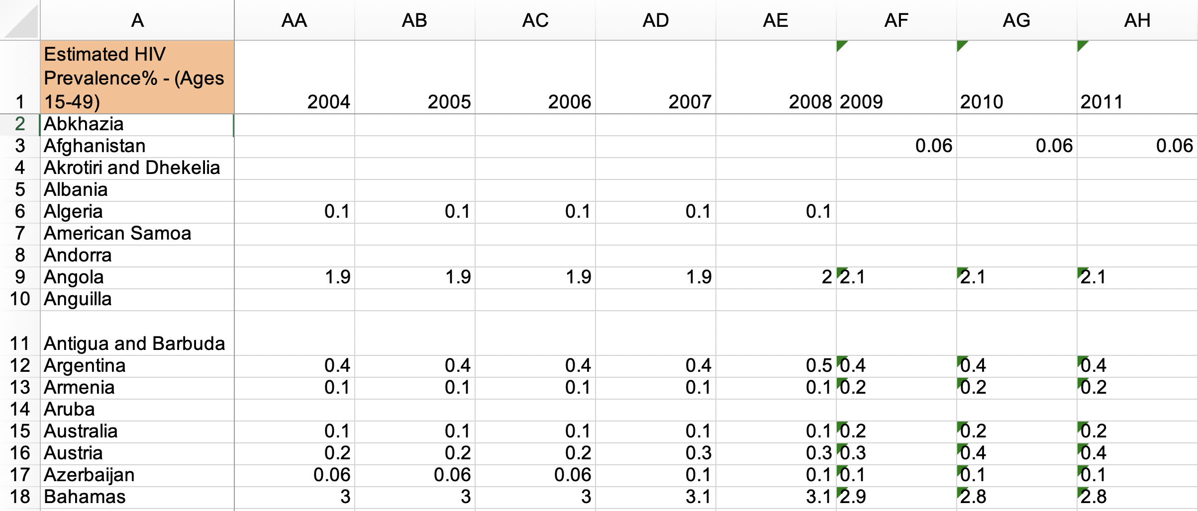
Examples of Untidy Data
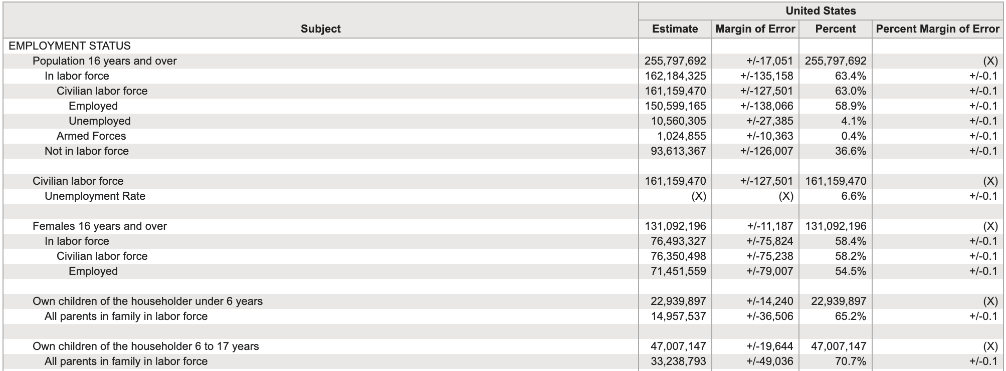
Examples of Untidy Data
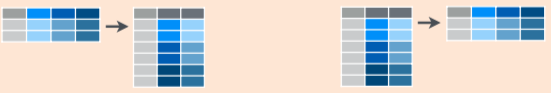
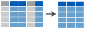
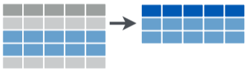
Reshaping/Pivoting Data
tidyrpackage helps reshape data into more usable formatMost common use: reshaping data between “long” and “wide”
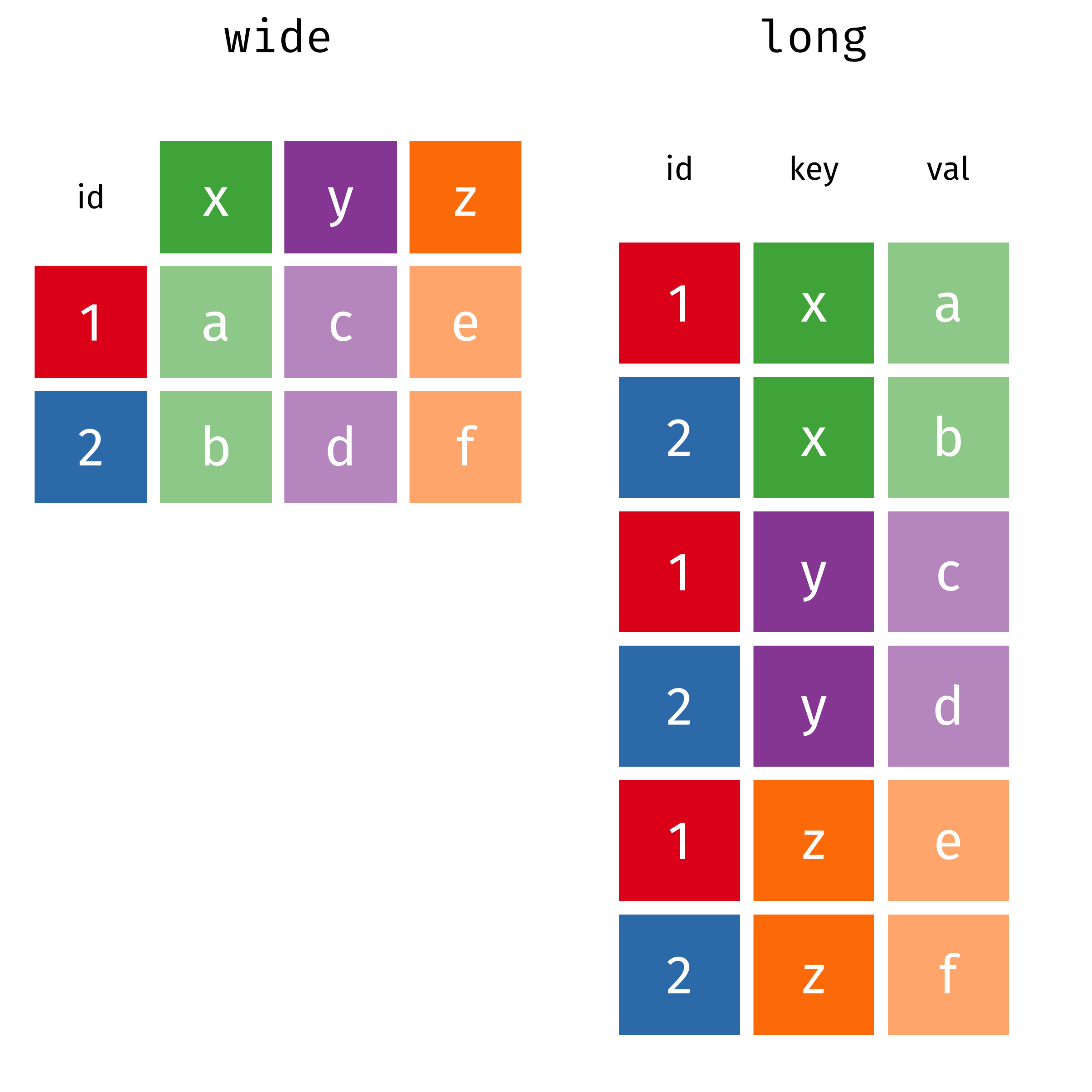
Reshaping
Source: Garrick Aden-Buie’s tidyexplain
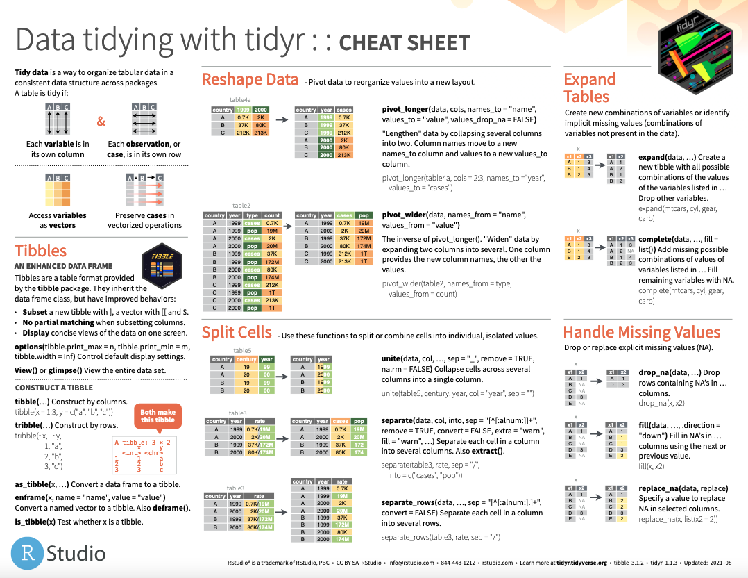
Data Tidying Cheat Sheet
dplyr I

dplyruses more efficient & intuitive commands to manipulate tibblesBase Rgrammar passively runs functions on nouns:function(object)dplyrgrammar actively uses verbs:verb(df, conditions)1
dplyr II
- Great features:
- Allows use of
%>%pipe operator - Input and output is always a
tibble - Shows the output from a manipulation, but does not save/overwrite as an object unless explicitly assigned to an object
- Several packages provide backends to SQL (
dbplyr), Apache Spark (sparklyr)
- Allows use of
dplyr Verbs
- Common
dplyrverbs
| Verb | Does |
|---|---|
filter() |
Keep only selected observations |
select() |
Keep only selected variables |
arrange() |
Reorder rows (e.g. in numerical order) |
mutate() |
Create new variables |
summarize() |
Collapse data into summary statistics |
group_by() |
Perform any of the above functions by groups/categories |
select() Variables
filter() Select Rows by Condition
mutate(): Create New Variables

summarize(): Create Statistics

Piping Across Packages
tidyverseuses same grammar and design philosophy
gapminder %>%
  group_by(continent, year) %>%
  summarize(mean_life = mean(lifeExp),
            mean_GDP = mean(gdpPercap)) %>%
  # now pipe this tibble in as data for ggplot!
  ggplot(data = ., # . pipes the above in (to data layer)
         aes(x = year,
             y = mean_life,
             color = continent))+
  geom_path(size = 1)+
  labs(x = "Year",
       y = "Average Life Expectancy (Years)",
       color = "Continent",
       title = "Average Life Expectancy Over Time")+
  theme_classic(base_family = "Fira Sans Condensed",
                base_size = 20)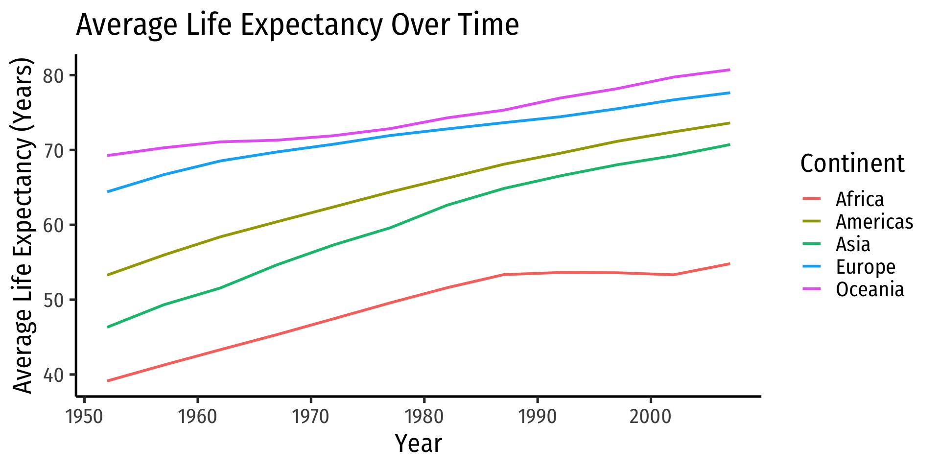
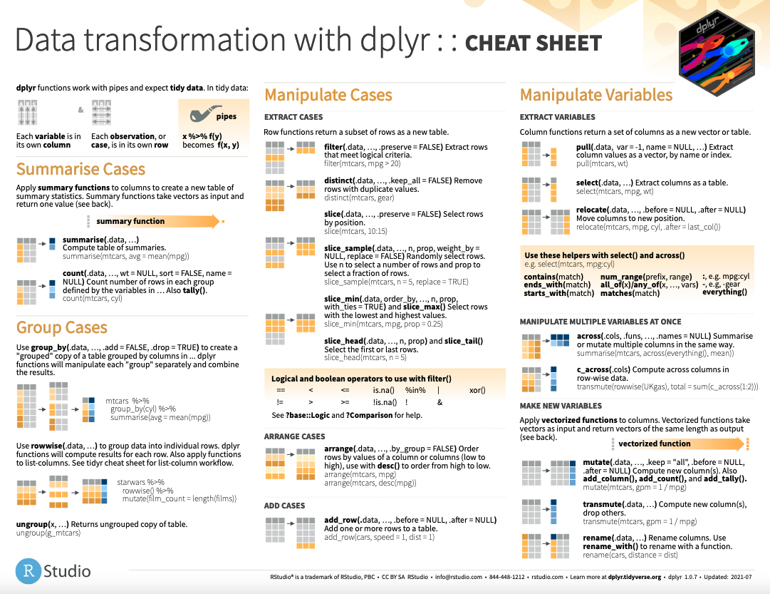
Data Wrangling Cheat Sheet
Resources
- R For Data Science, Chapter 10: Tibbles
- R For Data Science, Chapter 11: Data Import
- R Studio Cheatsheet: Data Import
- R For Data Science, Chapter 5: Data Transformation
- R Studio Cheatsheet: Data Wrangling (New version)
- R For Data Science, Chapter 12: Tidy Data
- R Studio Cheatsheet: Data Wrangling
- R Studio Cheatsheet: Data Import
- R For Data Science, Chapter 13: Relational Data
- R Studio Cheatsheet: Data Transformation
