[1] 41.5 — Optimize Workflow
ECON 480 • Econometrics • Fall 2022
Dr. Ryan Safner
Associate Professor of Economics
safner@hood.edu
ryansafner/metricsF22
metricsF22.classes.ryansafner.com
Your Workflow Has a Lot of Moving Parts
Writing text/documents
Managing citations and bibliographies
Performing data analysis
Making figures and tables
Saving files for future use
Monitoring changes in documents
Collaborating and sharing with others
Combining into a deliverable (report, paper, presentation, etc.)

The Office Model
The Office Model I
Writing text/documents
Managing citations and bibliographies
Performing data analysis
Making figures and tables
Saving files for future use
Monitoring changes in documents
Collaborating and sharing with others
Combining into a deliverable (report, paper, presentation, etc.)
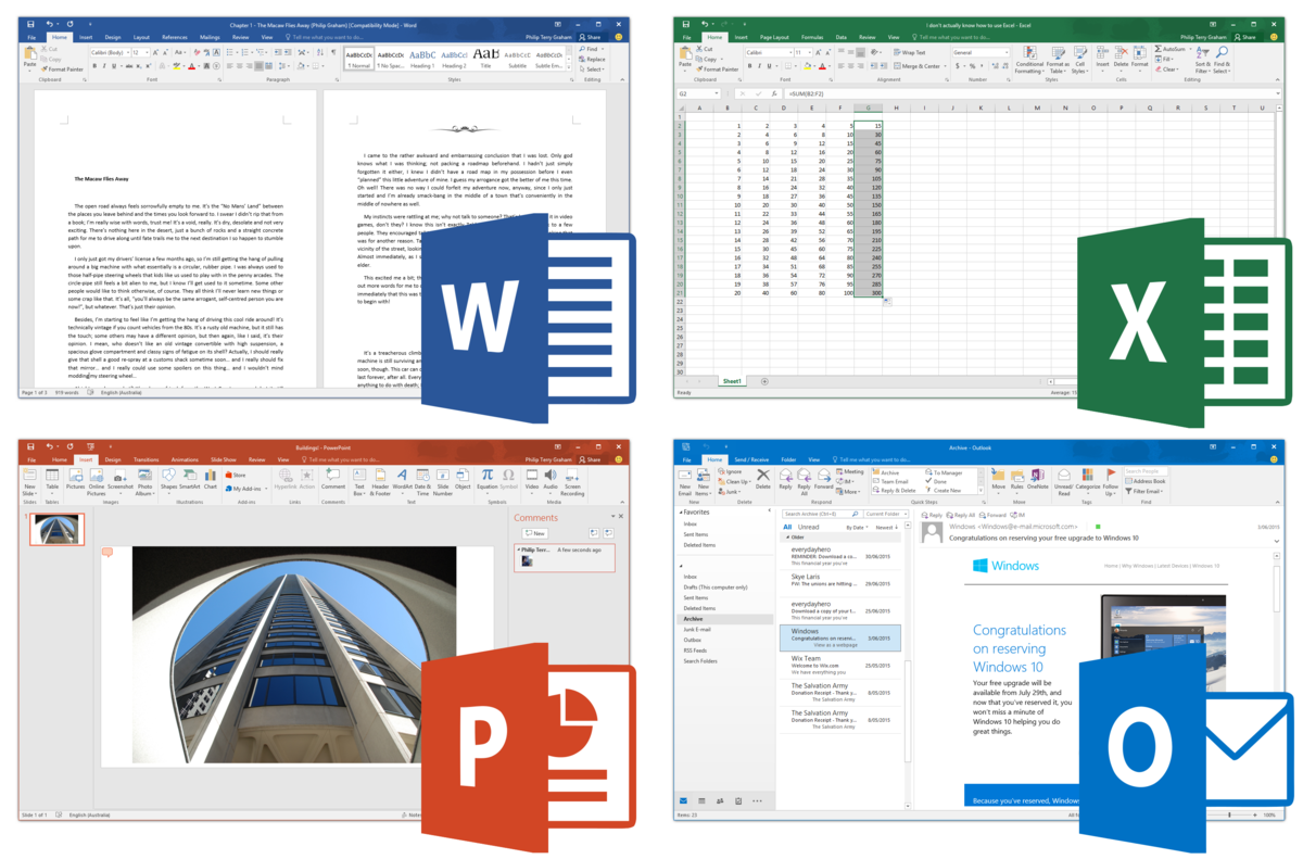
The Office Model II
A lot of copy/paste
A lot of:
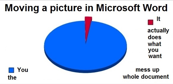

The Office Model: A Short Horror Film
The Office Model: Mistakes
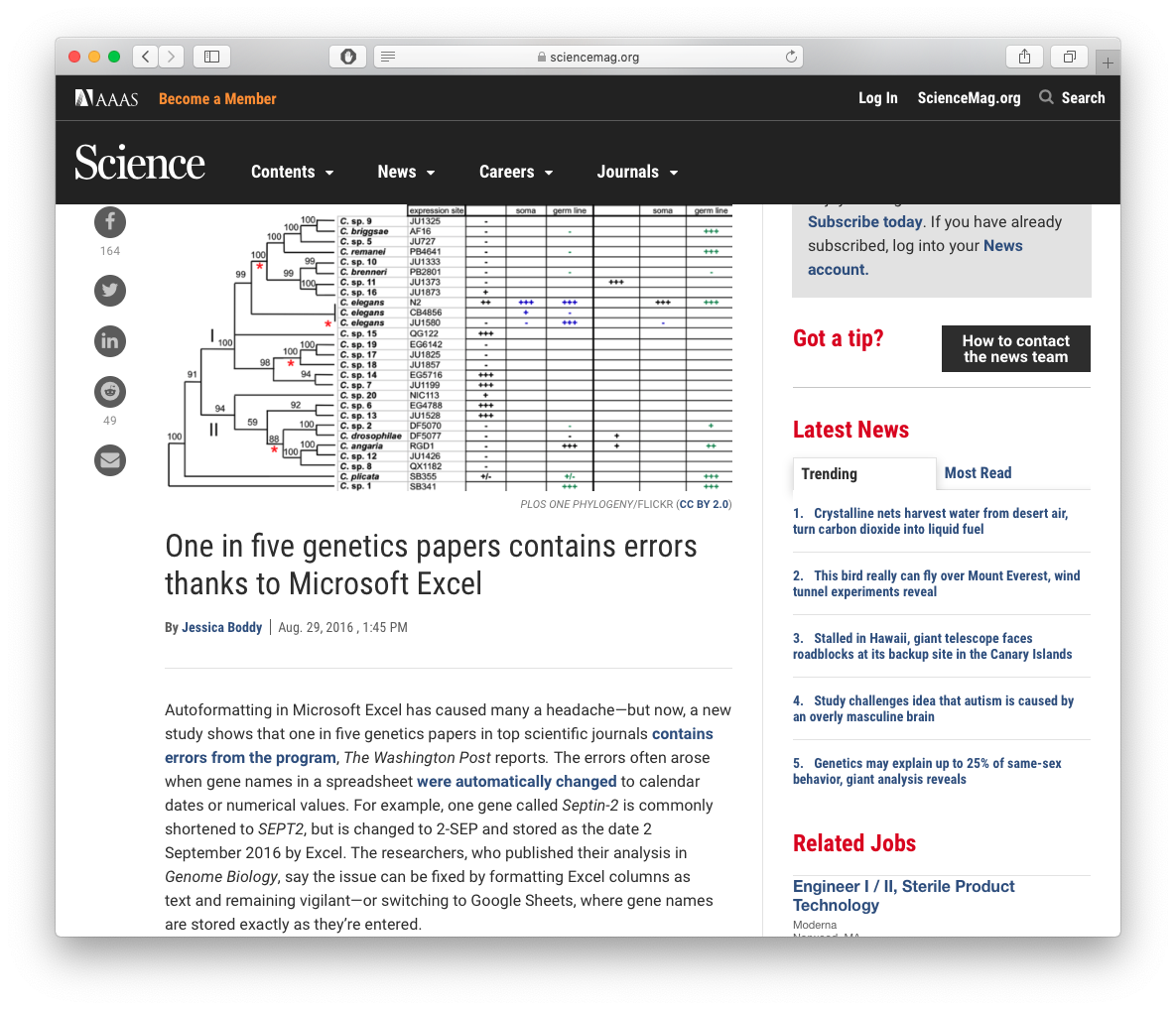
Source: Science Magazine
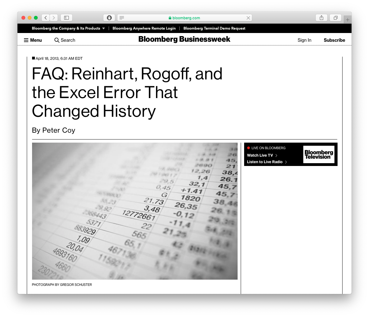
Source: Bloomberg
The Office Model: Not Reproducible
"'Reproducible research' is a redundant term. 'Irreproducible research' just used to be known as 'bullshit'." - @fperez_org ::slow clap::
— Kaitlin Thaney 💁🏻 (@kaythaney) May 8, 2014
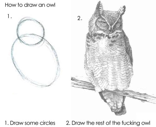
Drawing the Rest of the Owl
What I’ll Show You
This is how I make my…
- Research papers
- Course documents
- Websites
- Slides and presentations
I have not used any MS Office products since 2011 (good riddance!)
This stuff is optional
- If you like your office model, you can keep it
- But this is what most people who take this course continue to use (R is only really if you have data work)
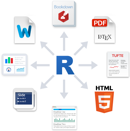
The Plain Text Model
The Plain Text Model II
Meet Quarto, which can do all of this in one pipeline
Writing text/documents
Managing citations and bibliographies
Performing data analysis
Making figures and tables
Saving files for future use
Monitoring changes in documents
Collaborating and sharing with others
Combining into a deliverable (report, paper, presentation, etc.)
The Plain Text Model II
- Plain text files: readable by both machines and humans
- Understand how a document is structured and formatted via code and markup to text
- Focus entirely on the actual writing of the content instead of the formatting and aesthetics
- You can still customize, but with precise commands instead of point, click, drag, guess, pray

The Plain Text Model III
Open Source: free, useable forever, often very small file size
- Proprietary software is a gamble - can you still open a
.docfile from Microsoft Word 1997?
- Proprietary software is a gamble - can you still open a
Automate and Minimize Errors, especially in repetitive processes
Can be used with version control (see below)

Making Your Work Reproducible
Quartofile (.qmd) is the “real” part of your analysis, everything can live in this plain-text file!Document text in
markdownR codeexecuted in “chunks”Plots and tables generated from
R codeCitations and bibliography automated with
.bibfile

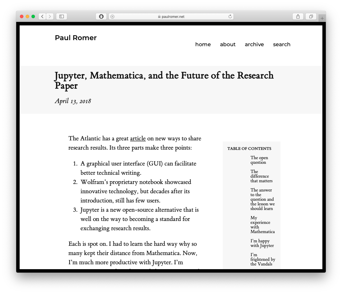
The Future of Science is Open Source Plain Text
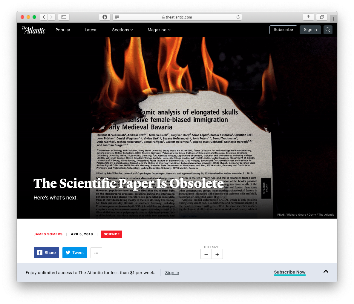
Source: The Atlantic
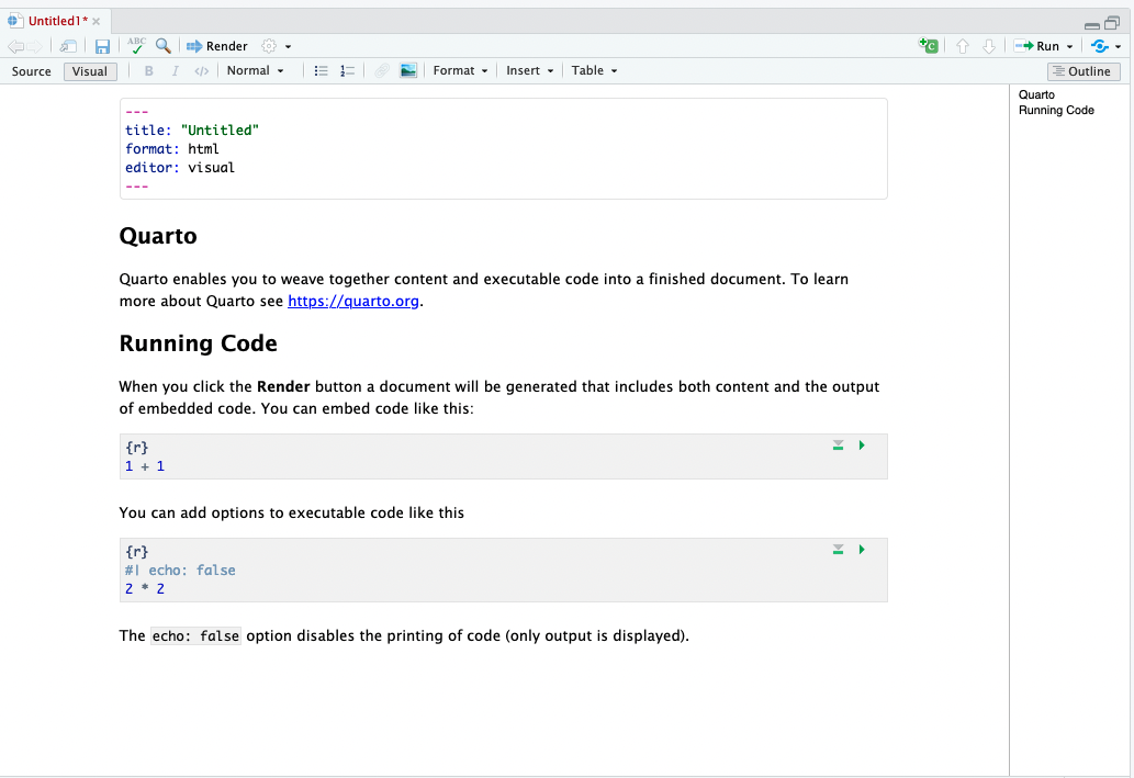
Quarto
Creating a Quarto Document I
File -> New File -> Quarto Document...
- Outputs:
- Document (what you’ll use for most things)
- Presentation (for making slides in various formats)
- Interactive (an html and R based web app, advanced)
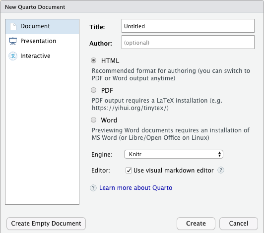
Creating a Quarto Document I
html: renders a webpage, viewable in any browser- default, easiest to produce and share
- can have interactive elements (gifs, animations, web apps)
- requires internet connection to host and share (you can view offline)
pdf: renders a PDF document- most common document format around
- requires
LaTeXdistribution to render (more on that soon)
word: create a Micosoft Word document- …if you must

Structure of a Quarto Document
YAML Header I
Top of a document contains the
YAML1 separated by three dashes---above and belowContains the metadata of the document, such as:
formatmust be specified, everything else can be left blank, and other options can be added as necessaryIn most cases, you can safely ignore other things in the
yamluntil you are ready
YAML Header Example I
- Example from these slides
YAML Header Example II
- Example from one of my papers:
---
title: Distributing Patronage^[I would like to thank the Board of Associates of Hood College...]
subtitle: Intellectual Property in the Transition from Natural State to Open Access Order
date: \today
author:
- Ryan Safner^[Hood College, Department of Economics and Business Administration; safner@hood.edu]

abstract: |
  | "This paper explores the emergence of the modern forms of copyright and patent in ...
  | *JEL Classification:* O30, O43, N43
  | *Keywords:* Copyright, intellectual property, economic history, freedom of the press, economic development

bibliography: patronage.bib
geometry: margin = 1in
fontsize: 12pt
mainfont: Fira Sans Condensed
output:
  pdf_document:
    latex_engine: xelatex
    number_sections: true
    fig_caption: yes

header-includes:
    - \usepackage{booktabs}
---
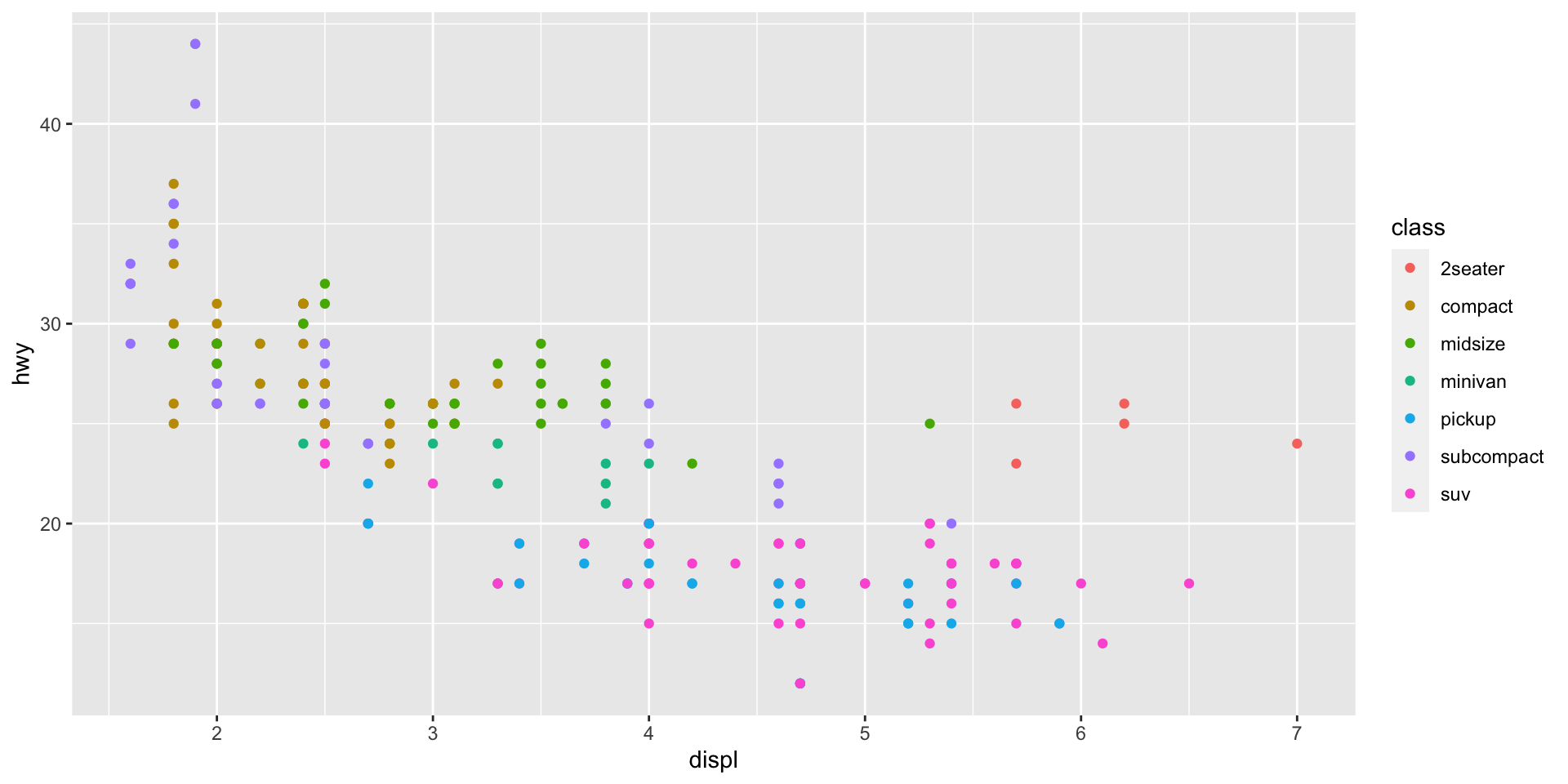
R Chunks
- You can create a “chunk” of
Rcode with three backticks1 above and below your code - After the first pair of backticks, signify the language of the code2 inside braces, e.g:
R Chunks
Output
# A tibble: 6 × 6
  country     continent  year lifeExp      pop gdpPercap
  <fct>       <fct>     <int>   <dbl>    <int>     <dbl>
1 Afghanistan Asia       1952    28.8  8425333      779.
2 Afghanistan Asia       1957    30.3  9240934      821.
3 Afghanistan Asia       1962    32.0 10267083      853.
4 Afghanistan Asia       1967    34.0 11537966      836.
5 Afghanistan Asia       1972    36.1 13079460      740.
6 Afghanistan Asia       1977    38.4 14880372      786.
R Chunks
R Chunk Options
- Chunks can have options with the “hash pipe”
#|at the top of the chunk
Global Chunk Options
- You can set default options for all chunks in the
YAMLheader:
R Inline Code
- If you just want to display some code (or at least format it like code) in the middle of a sentence, place between a single backtick on either side.
- e.g. if I mention
`tidyverse`or`gapminder`, it formats the text asin-line code.
- e.g. if I mention
- To actually execute
Rcode to output something in the middle of a sentence, putras the first character inside the backticks, and then run the actual code such as pi is equal to 3.1415927.
Input
pi is equal to `r pi`.
Output
pi is equal to 3.1415927.
Or Like This
Input
The average GDP per capita is ` r dollar(mean(gapminder$gdpPercap)) ` with a standard deviation of ` r dollar(sd(gapminder$gdpPercap)) `.
Output
The average GDP per capita is $7,215.33 with a standard deviation of $9,857.45.
Writing Text with Markdown: Formatting
- Markdown is a lightweight markup language geared towards HTML (i.e. the internet)
- Markup languages used to add commands about how to display plain text
| Markdown Syntax | Output |
|---|---|
|
italics and bold |
|
superscript2 / subscript2 |
|
|
|
verbatim code |
- Comment your document with
<!-- Unprinted comments here -->(will not print in output; this comes fromhtml)
Writing Text with Markdown: Lists
| Markdown Syntax | Output |
|---|---|
|
|
|
|
|
|
Writing Text with Markdown: Headings
| Markdown Syntax | Output |
|---|---|
|
Header 1 |
|
Header 2 |
|
Header 3 |
|
Header 4 |
|
Header 5 |
|
Header 6 |
Writing Text with Markdown: Links
Markdown
Output
You can embed named hyperlinks, direct urls like https://metricsF22.classes.ryansafner.com/, and links to other places — like the previous slide in the document.
Writing Text with Markdown: Images
Output


- Read the Quarto Documentation on figures for more.
Writing Text with Markdown: Making Tables
Markdown
| Right | Left | Default | Center |
|------:|:-----|---------|:------:|
|   12  |  12  |    12   |    12  |
|  123  |  123 |   123   |   123  |
|    1  |    1 |     1   |     1  |

: Table Example {tbl-colwidths="[25,25,25,25]"}
Output
| Right | Left | Default | Center |
|---|---|---|---|
| 12 | 12 | 12 | 12 |
| 123 | 123 | 123 | 123 |
| 1 | 1 | 1 | 1 |
- See the Quarto Documentation for more help on tables
Writing Text with Markdown: Printing Tables
- Sometimes we want to print tables from our data
- The
kableExtrapackage is great for this see Documentation
| mpg | cyl | disp | hp | drat | wt | qsec | vs | am | gear | carb | |
|---|---|---|---|---|---|---|---|---|---|---|---|
| Mazda RX4 | 21.0 | 6 | 160 | 110 | 3.90 | 2.620 | 16.46 | 0 | 1 | 4 | 4 |
| Mazda RX4 Wag | 21.0 | 6 | 160 | 110 | 3.90 | 2.875 | 17.02 | 0 | 1 | 4 | 4 |
| Datsun 710 | 22.8 | 4 | 108 | 93 | 3.85 | 2.320 | 18.61 | 1 | 1 | 4 | 1 |
| Hornet 4 Drive | 21.4 | 6 | 258 | 110 | 3.08 | 3.215 | 19.44 | 1 | 0 | 3 | 1 |
| Hornet Sportabout | 18.7 | 8 | 360 | 175 | 3.15 | 3.440 | 17.02 | 0 | 0 | 3 | 2 |
| Valiant | 18.1 | 6 | 225 | 105 | 2.76 | 3.460 | 20.22 | 1 | 0 | 3 | 1 |
Writing Text with Markdown: Printing Tables
Writing Math
- Add beautifully-formatted math with the
$tag before and after the math, two$$before/after for a centered equation
- In-line math example:
$1^2=\frac{\sqrt{16}}{4}$produces \(1^2=\frac{\sqrt{16}}{4}\) in my text
- Centered-equation example:
Input
$$ \hat{\beta_1}=\frac{\displaystyle \sum_{i=1}^n (X_i-\bar{X})(Y_i-\bar{Y})}{\displaystyle \sum_{i=1}^n (X_i-\bar{X})^2} $$
Output
\[\hat{\beta_1}=\frac{\displaystyle \sum_{i=1}^n (X_i-\bar{X})(Y_i-\bar{Y})}{\displaystyle \sum_{i=1}^n (X_i-\bar{X})^2}\]
Writing Math
- Math uses a (much older) language called \(\LaTeX\), used by mathematicians, economists, and others to write papers and slides with perfect math and formatting
- I used to use for everything before I found
Randmarkdown - Producing
pdfoutput actually convertsmarkdownfiles into \(\TeX{}\) first! - Much steeper learning curve, a good cheatsheet
- An extensive library of mathematical symbols, notation, formats, and ligatures, e.g.
- I used to use for everything before I found
- A great resource: Wikibooks LaTeX Mathematics chapter
Writing Math
| Input | Output |
|---|---|
$\alpha$ |
\(\alpha\) |
$\pi$ |
\(\pi\) |
$\frac{1}{2}$ |
\(\frac{1}{2}\) |
$\hat{x}$ |
\(\hat{x}\) |
$\bar{y}$ |
\(\bar{y}\) |
$x_{1,2}$ |
\(x_{1,2}\) |
x^{a-1}$ |
\(x^{a-1}\) |
$\lim_{x \to \infty}$ |
\(\lim_{x \to \infty}\) |
$A=\begin{bmatrix} a_{1,1} & a_{1,2} \\ a_{2,1} & a_{2,2} \\ \end{bmatrix}$ |
\(A=\begin{bmatrix} a_{1,1} & a_{1,2} \\ a_{2,1} & a_{2,2} \\ \end{bmatrix}\) |
Citations, References, & Bibliography
- Manage your citations and bibliography automatically with
.bibfiles - First create a
.bibfile to list all of your references in- You can do this in
Rvia:File -> New File -> Text File(and save with.bibat the end) - See
examplebib.bibin this repository used in this document - At the top of your
YAMLheader in the main document, addbibliography: examplebib.bibsoRknows to pull references from this file - For each reference, add information to a
.bibfile, like so:
- You can do this in
An Example .bib File
A
.bibfile is a plain text file with entries like thisClasses for
@article,@book,@collectedwork,@unpublished, etc.- Each will have different keys needed (e.g.
editor,publisher,address)
- Each will have different keys needed (e.g.
First input after the
@articleis your citation key (e.g.safner2016)- Whenever you want to cite this article, you’ll invoke this key
Citations
Whenever you want to cite a work in your text, call up the citation key with
@, like so:@safner2016[], which produces (Safner, 2016)You can customize citations, e.g.:
| Write | Produces |
|---|---|
[@Safner2016] |
(Safner, 2016) |
@Safner2016 |
Safner 2016 |
-@Safner2016 |
(2016) |
@Safner2016[p. 743-744] |
(Safner, 2016, p.743-744) |
- BibTeX will automatically collect all works cited at the end and produce a bibliography according to a style you can choose
Reference Management Software
For more information and examples, see Quarto’s Documentation on Citations
Lot of programs can help you manage references and export complete
.bibfiles to use withR Markdown
Plain-Text Editors
Markdown files are plain text files and can be edited in any text editor
- something as basic (and boring!) as “Notepad,” for example
- many good text editors out there: Typora; Ulysses
Any good editor will have syntax highlighting and coloring when you use tags (like bold, italic,
code, andcode #comments).
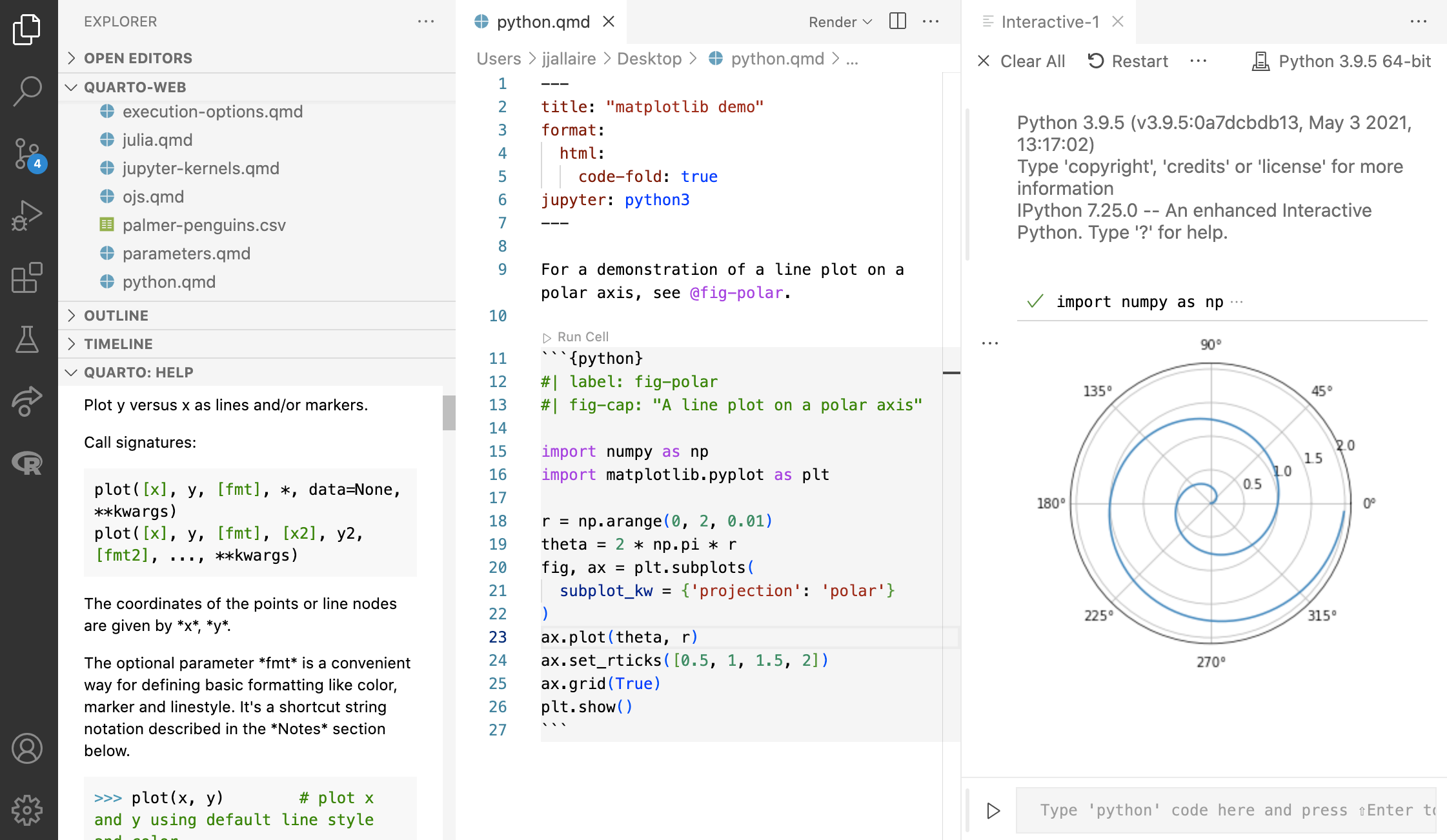
VS Code
RStudio is My Text Editor of Choice
- Honestly, I write everything in R Studio’s text editor
- Syntax highlighting
- Actually can run R code, autocomplete, etc
- Can render the markdown to an output format: html, pdf, etc.
- You can write R code in other text editors, but you can’t execute them outside of R Studio (or the command line, but that’s too advanced.) Same with actually rendering your markdown to an output (pdf, html, etc)
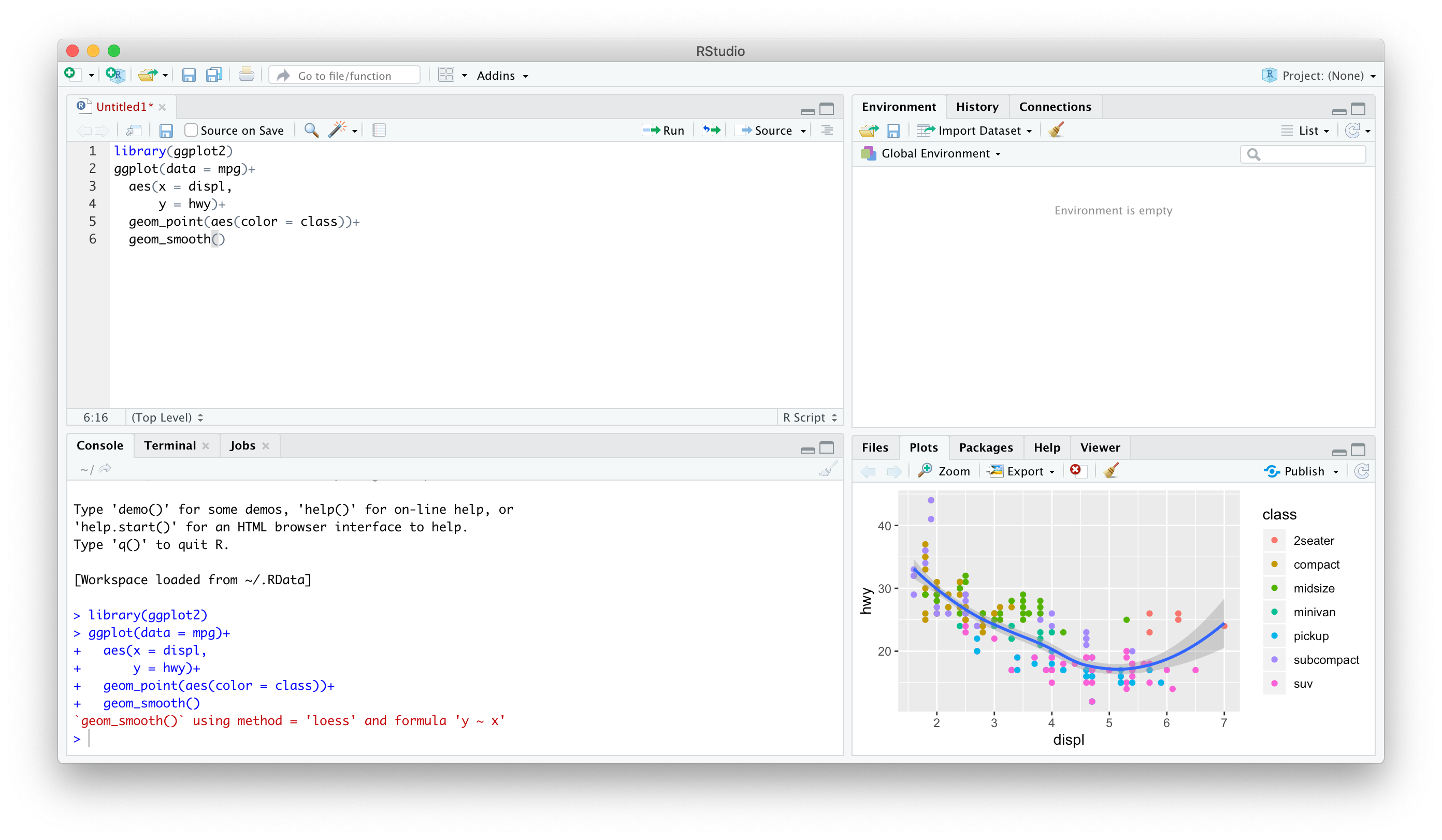
Tips with Markdown
Empty space is very important in markdown
Lines that begin with a space may not render properly
Math that contains spaces between the dollar-signs may not render properly
Moving from one type of content to another (e.g. a heading to a list to text to an equation to text) requires blank lines between them to work
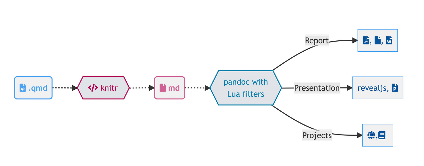
Rendering Your Documents
knitr
When you are ready, you “redner” your markdown and code into an output format using:
knitr1, an R package that “knits” your R code and markdown.qmdinto a.mdfile for:pandoc is a “swiss-army knife” utility that can convert between dozens of document types
All you need to do is click the
Renderbutton at the top of the text editor!
PDF Output
Producing a PDF uses \(\LaTeX{}\)
You will need a full distribution of \(\LaTeX{}\) on your computer, OR
- Better to use the package
tinytexto install a mini-distro of \(\LaTeX{}\) inside ofR:
Project-Oriented Workflow
R Projects I
- A
R Projectis a way of systematically organizing yourRhistory, working directory, and related files in a single, self-contained directory - Can easily be sent to others who can reproduce your work easily
- Connects well with version control software like GitHub
- Can open multiple projects in multiple windows
R Projects I
- Projects solve all of the following problems:
- Organizing your files (data, plots, text, citations, etc)
- Having an accessible working directory (for loading and saving data, plots, etc)
- Saving and reloading your commands history and preferences
- Sending files to collaborators, so they have the same working directory as you

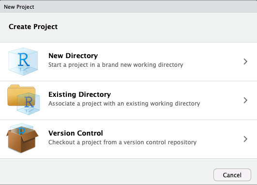
Creating an R Project I

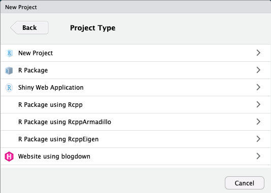
Creating an R Project II
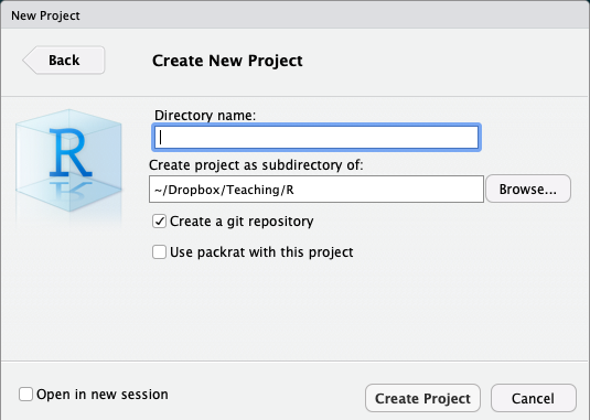
Creating an R Project III
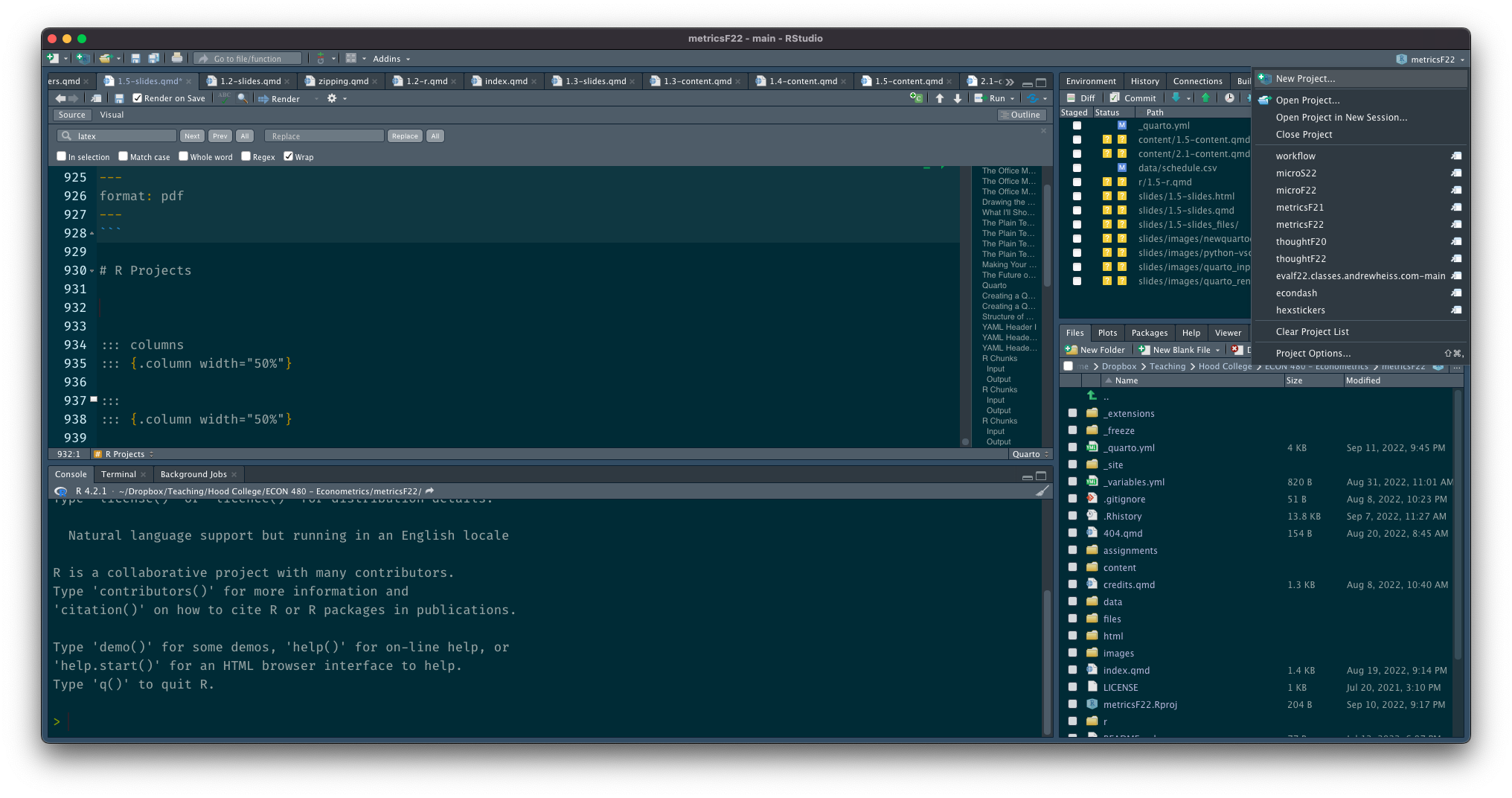
Projects
- Switch between each project (Window) on your computer (this is on a Mac)

Projects
- At top right corner of RStudio
- Click the button to the right of the name to open in a new window!
Loading Others’ Projects
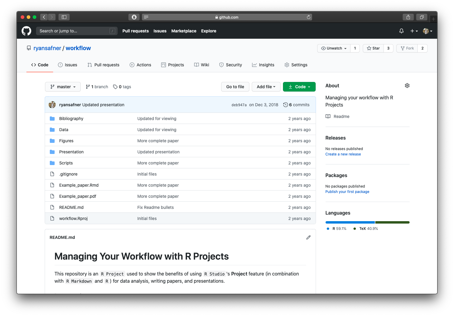
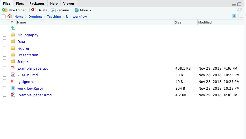
A Good File Structure
- Look through this on your own
- Read the
READMEof this repository on GitHub for instructions (automatically shows on the main page) - Look at the
example_paper.qmd- Uses data from data folder
- Uses
.Rscripts from scripts folder - Uses figures from figures folder
- Uses
bibexample.bibfrom bibliography folder
Version Control
Have You Done This?
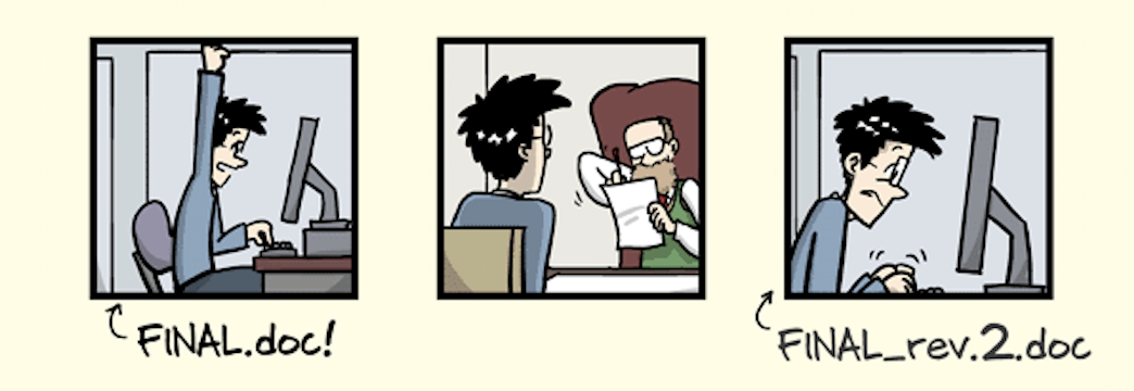
Source: PhD Comics
Have You Done This?
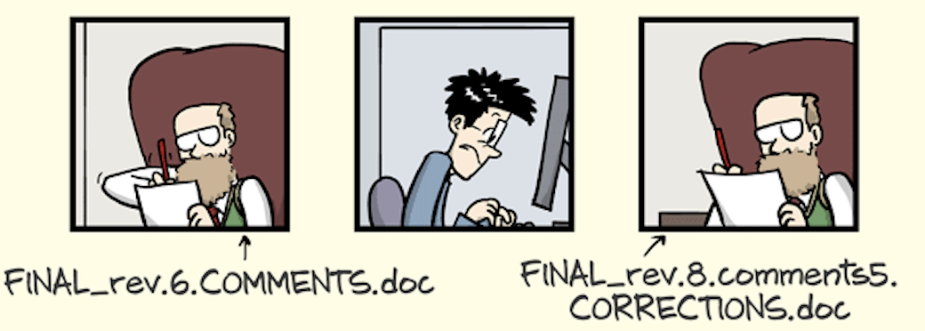
Source: PhD Comics
Have You Done This?
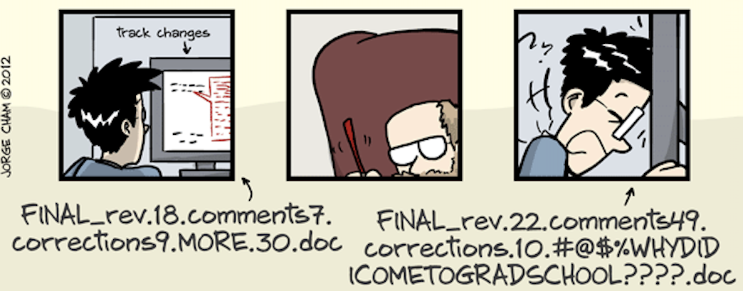
Source: PhD Comics
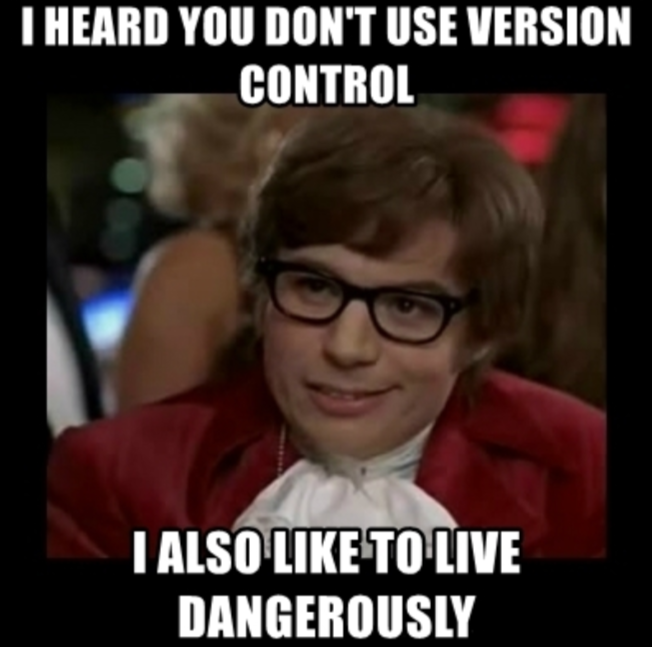
Do You Want to Be Able to
Keep your files backed up
Track changes
Collaborate on the same files with others
Edit files on one computer and then open and continue working on another?
The Training-Wheels Version
Register an account for free
Set up a location on your computer for the
Dropbox/folderAnything you put in this folder will sync to the cloud
- As soon as you change files, they automatically update and sync!
- Can download any of these flies from the website on any device
- Set this up on multiple computers so when you change a file on one, it updates on all the others!
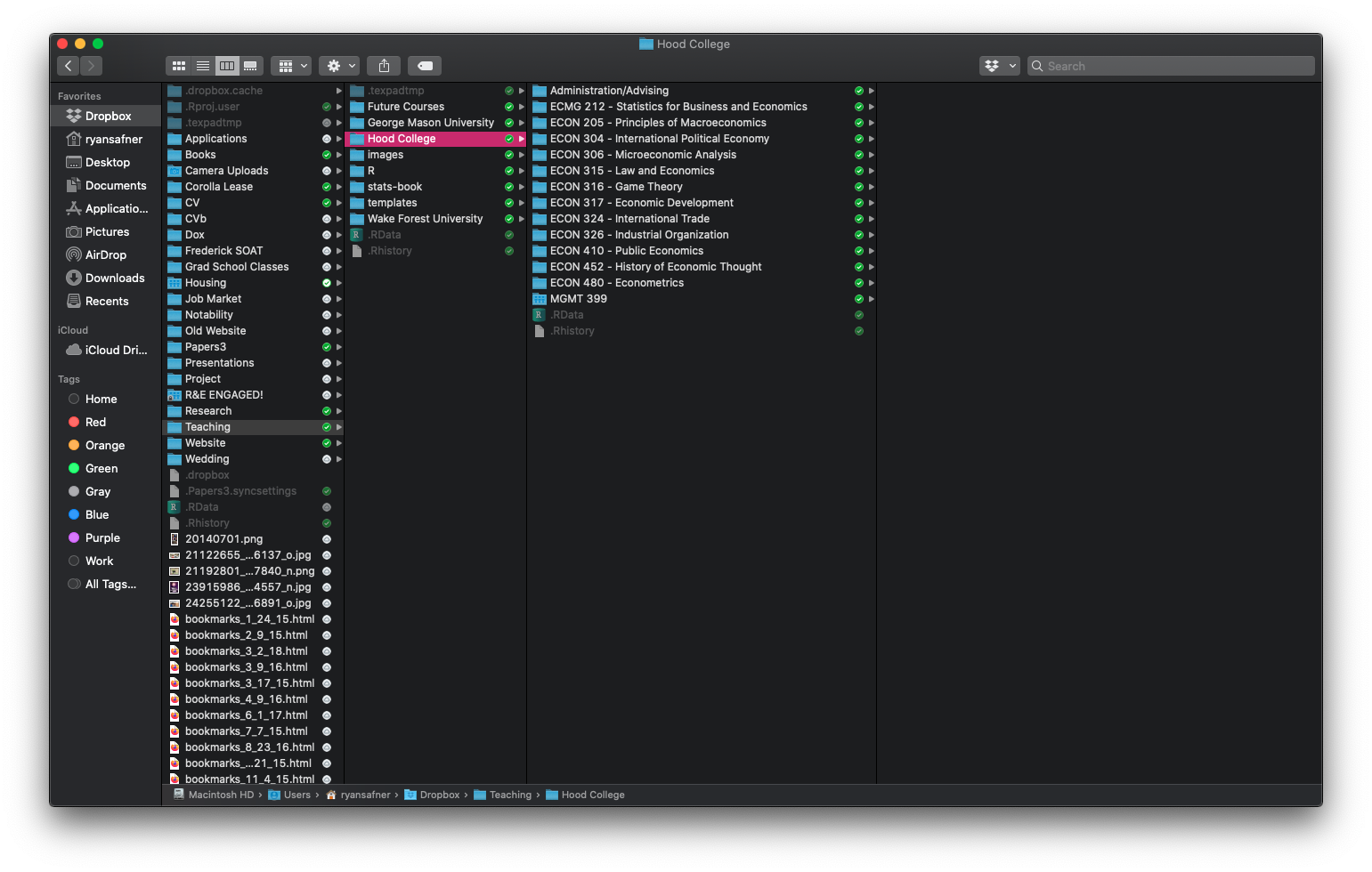
My Life Goes In Here
Smart Sync
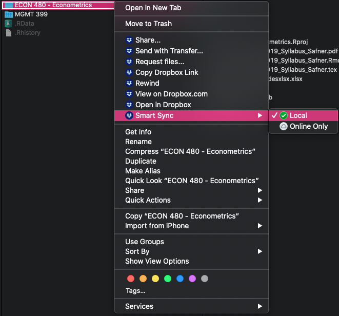
Smart Sync - keep some files online only for space
The Expert Version


Gitis an “open source distributed version control system” widely used in the software development industryTrack changes on steroids (if MS Word’s Track Changes and Dropbox had a baby)
- Organize folders/files to track (a
"repository") - Take a snapshot of all of your files (a “
commit”) with “comments” pushthese to the cloudpullchanges to (other) computers as needed
- Organize folders/files to track (a
GitHubis a popular (not the only!) cloud destination for these repositories
The Expert Version
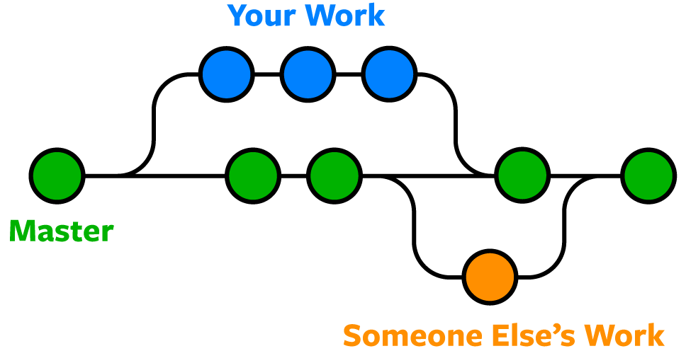
- Shows history (
versions) of files with comments- Can
forkorbranchrepository into multiple versions at once - Good for “testing” things out without destroying old versions!
revertback to original versions as needed
- Can
The Expert Version
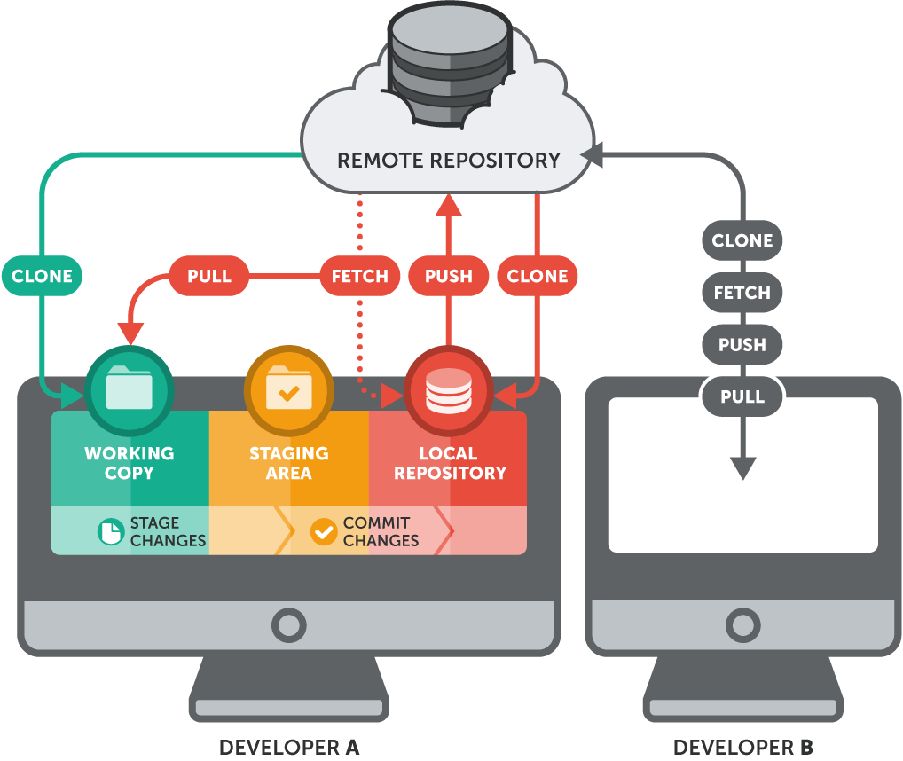
The Expert Version
Requires some advanced set up, see this excellent guide
R Studio integrates git and github commands nicely
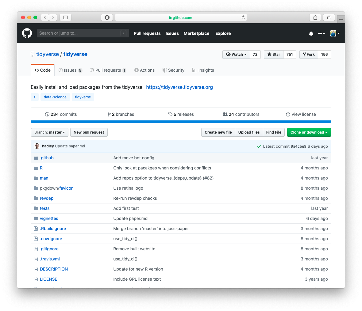
This Class on Github
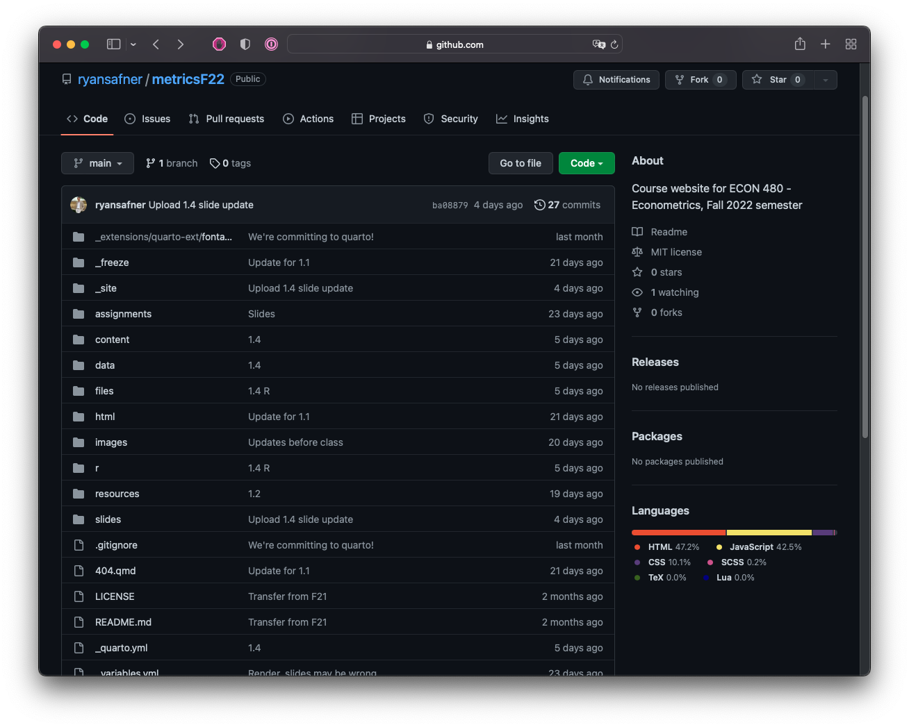

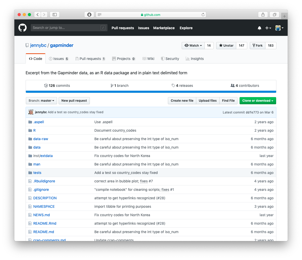
Most Packages Start on Github
My Workflow (That I Suggest to You)
- Create a new repository on Github.1
- Start a New R Project in R Studio (link it to the github repository - see guide)
- Create a logical file system (see example), such as:
project # folder on my computer (the new working directory)
|
|- data/ # folder for data files
|- scripts/ # folder .R code
|- bibliography/ # folder for .bib files
|- figures/ # folder to plots and figures to
|- paper.qmd # write document here- Write document in
paper.qmd, loading/saving files from/to various folders in project- e.g. load data like
df <- read_csv("data/my_data"); save plots likeggsave("figures/p.png")
- e.g. load data like
- Render document to
pdforhtml. - Occasionally,
stageandcommitchanges with a description,pushto GitHub.
Resources
- Quarto Documentation: Tutorial: Hello, Quarto
- Quarto Documentation: Tutorial: Computation
- Quarto Documentation: Tutorial: Authoring
- Quarto Documentation: Guide
- Kieran Healey’s The Plain Person’s Guide to Plain Text Social Science on managing workflow with plain text files, R, and Git
- Hadley Wickham’s (and Garrett Grolemund) R for Data Science on how to use R and R Markdown for data science work
- Jenny Bryan’s Happy Git with R on how to use git and GitHub with R as a version control system


