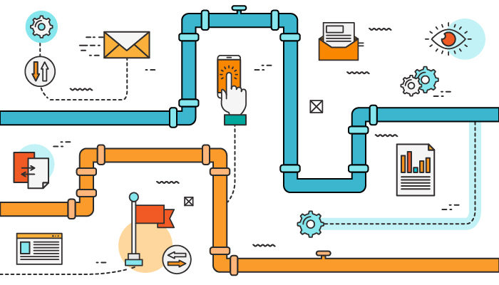
[1] 4Your Workflow Has a Lot of Moving Parts
Writing text/documents
Managing citations and bibliographies
Performing data analysis
Making figures and tables
Saving files for future use
Monitoring changes in documents
Collaborating and sharing with others
Combining into a deliverable (report, paper, presentation, etc.)
The Office Model I
Writing text/documents
Managing citations and bibliographies
Performing data analysis
Making figures and tables
Saving files for future use
Monitoring changes in documents
Collaborating and sharing with others
Combining into a deliverable (report, paper, presentation, etc.)
The Office Model II
A lot of copy/paste
A lot of:
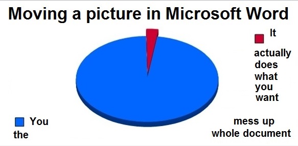
The Office Model: Mistakes
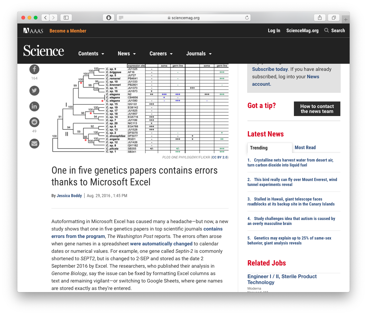
Source: Science Magazine
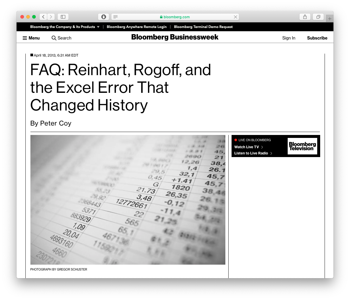
Source: Bloomberg
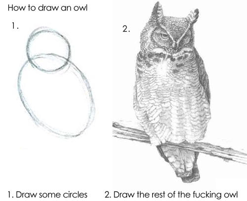
Drawing the Rest of the Owl
What I’ll Show You
This is how I make my…
- Research papers
- Course documents
- Websites
- Slides and presentations
I have not used any MS Office products since 2011 (good riddance!)
This stuff is optional
- If you like your office model, you can keep it
- But this is what most people who take this course continue to use (R is only really if you have data work)
The Plain Text Model II
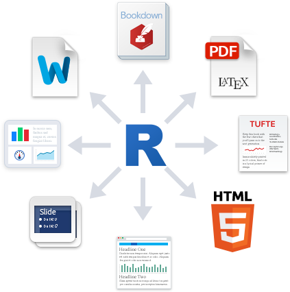
Meet Quarto, which can do all of this in one pipeline
Writing text/documents
Managing citations and bibliographies
Performing data analysis
Making figures and tables
Saving files for future use
Monitoring changes in documents
Collaborating and sharing with others
Combining into a deliverable (report, paper, presentation, etc.)
The Plain Text Model II
- Plain text files: readable by both machines and humans
- Understand how a document is structured and formatted via code and markup to text
- Focus entirely on the actual writing of the content instead of the formatting and aesthetics
- You can still customize, but with precise commands instead of point, click, drag, guess, pray
The Plain Text Model III
Open Source: free, useable forever, often very small file size
- Proprietary software is a gamble - can you still open a
.docfile from Microsoft Word 1997?
- Proprietary software is a gamble - can you still open a
Automate and Minimize Errors, especially in repetitive processes
Can be used with version control (see below)
Making Your Work Reproducible
Quartofile (.qmd) is the “real” part of your analysis, everything can live in this plain-text file!Document text in
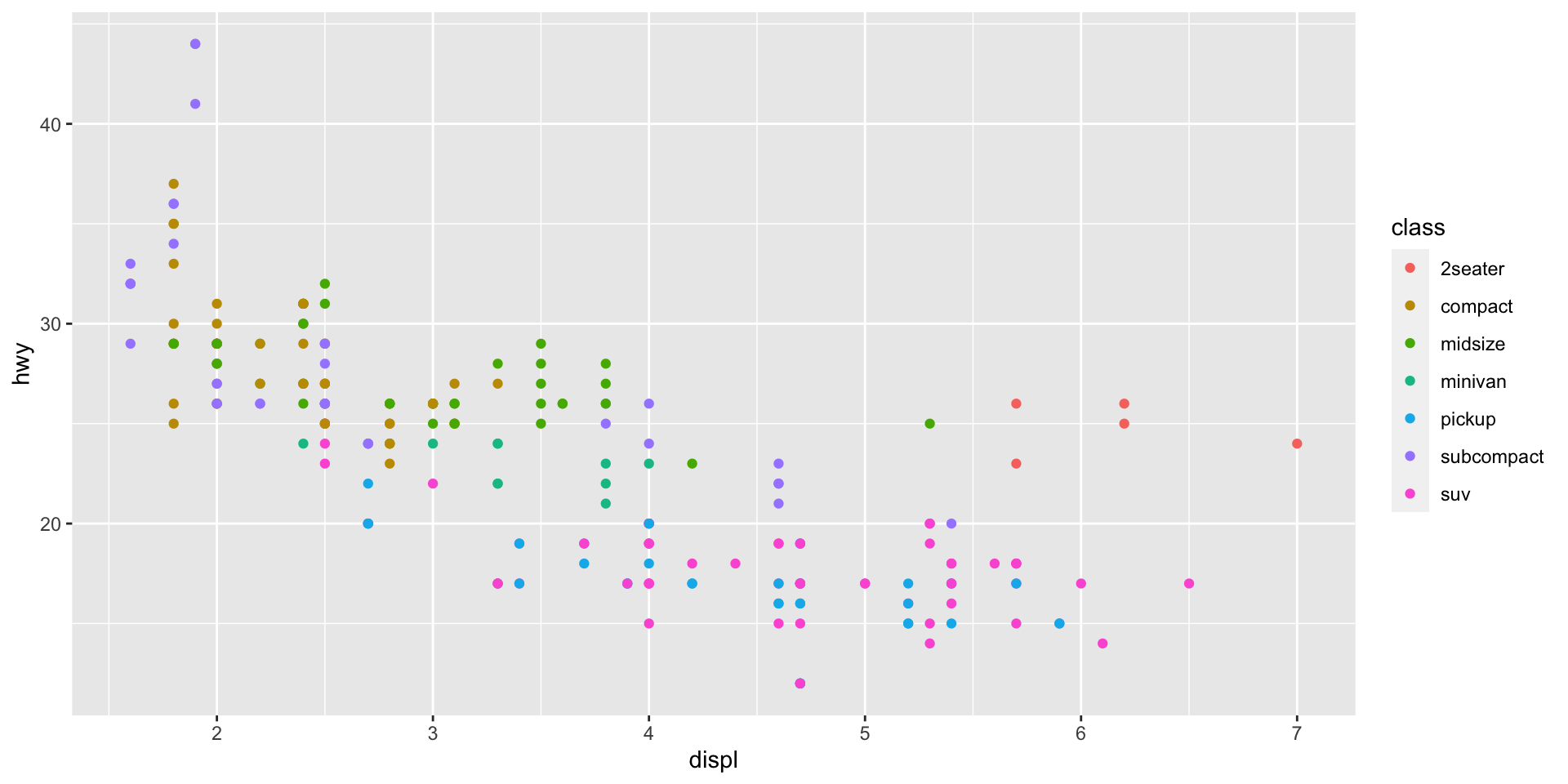
markdownR codeexecuted in “chunks”Plots and tables generated from
R codeCitations and bibliography automated with
.bibfile

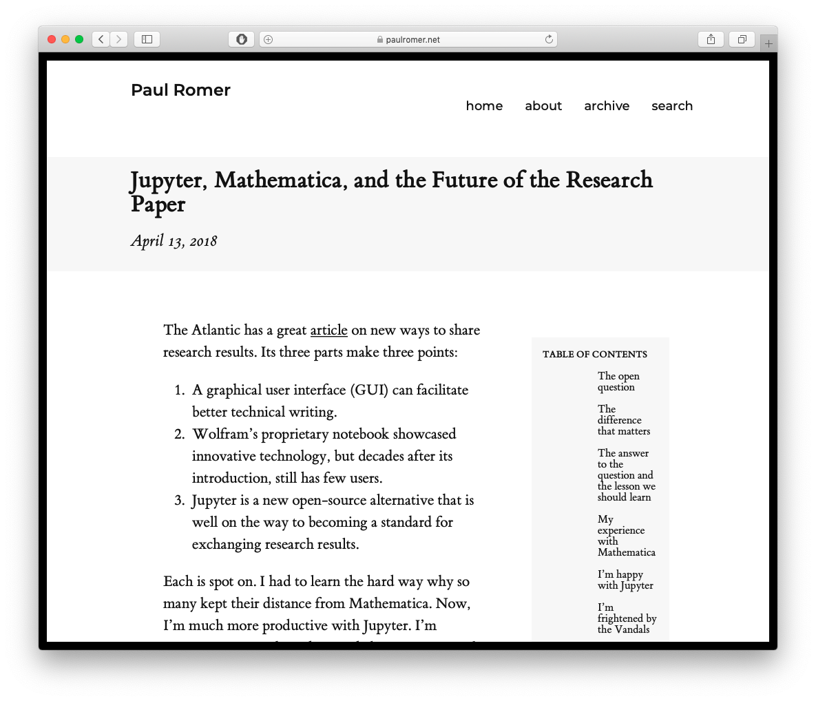
The Future of Science is Open Source Plain Text
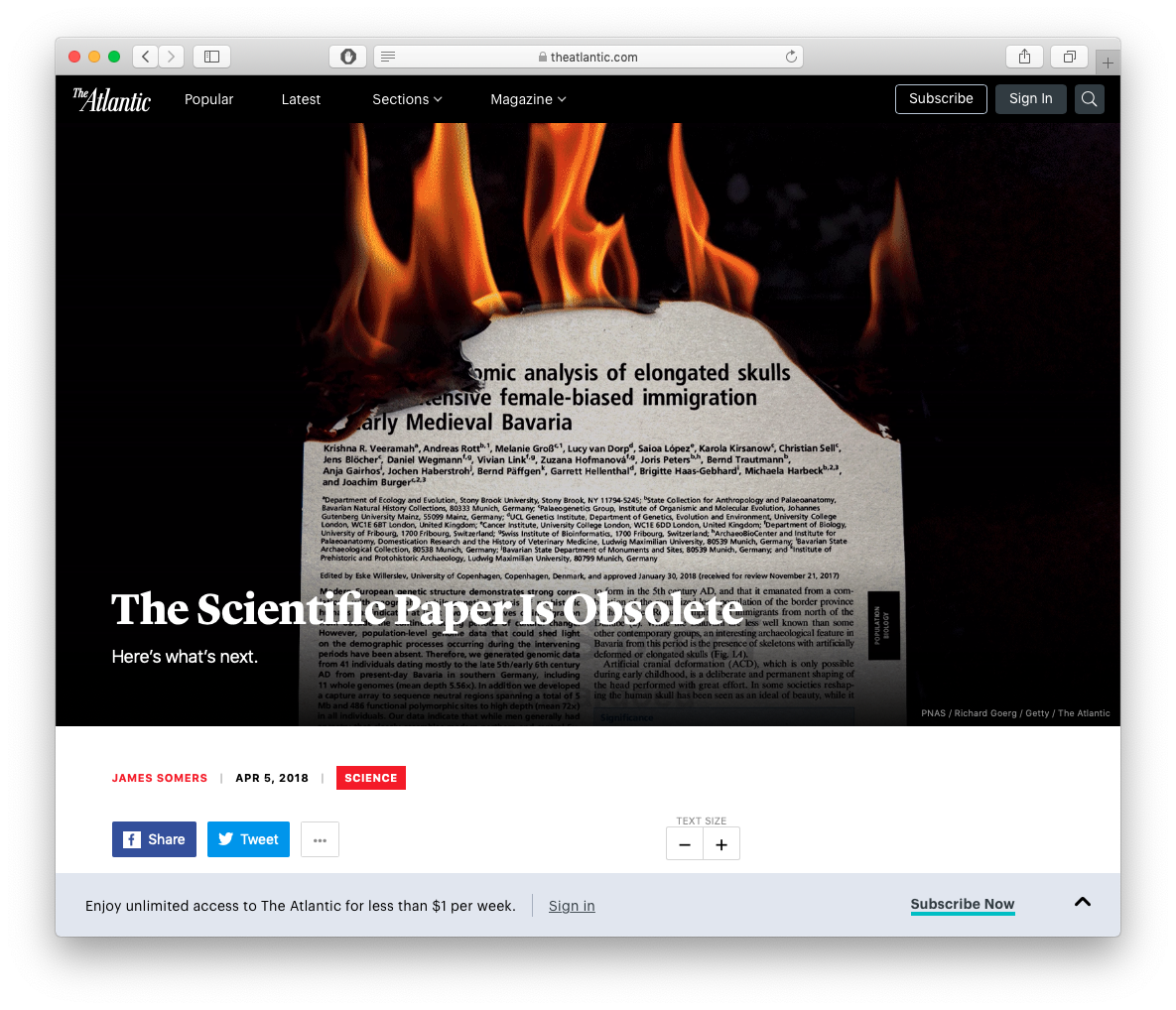
Source: The Atlantic
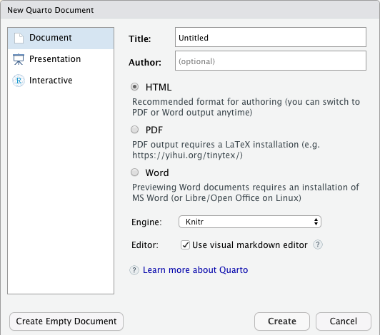
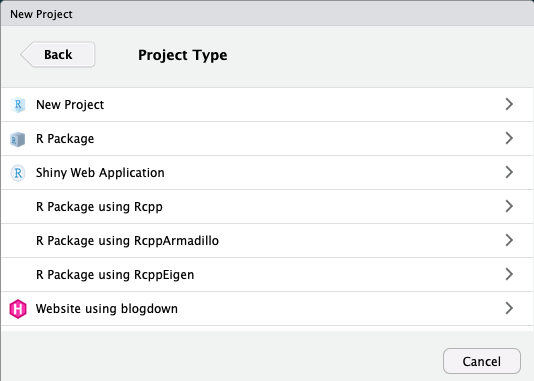
Creating a Quarto Document I
File -> New File -> Quarto Document...
- Outputs:
- Document (what you’ll use for most things)
- Presentation (for making slides in various formats)
- Interactive (an html and R based web app, advanced)
Creating a Quarto Document I
html: renders a webpage, viewable in any browser- default, easiest to produce and share
- can have interactive elements (gifs, animations, web apps)
- requires internet connection to host and share (you can view offline)
pdf: renders a PDF document- most common document format around
- requires
LaTeXdistribution to render (more on that soon)
word: create a Micosoft Word document- …if you must
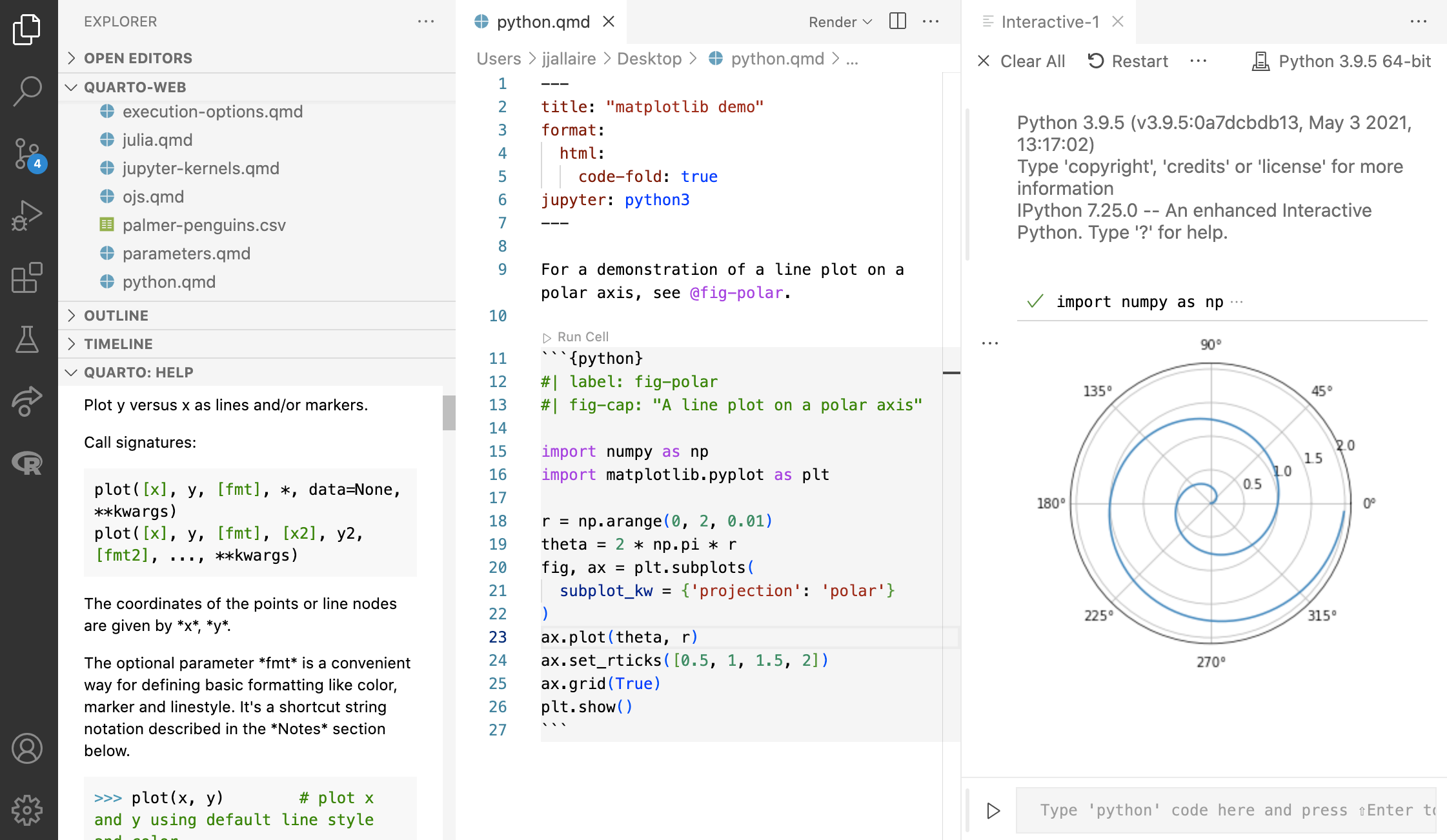
Structure of a Quarto Document
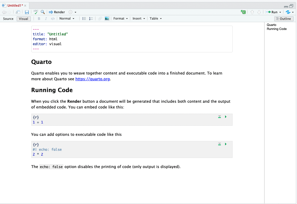
R Chunks
Writing Text with Markdown: Images
Output
![]()
- Read the Quarto Documentation on figures for more.
Plain-Text Editors
Markdown files are plain text files and can be edited in any text editor
- something as basic (and boring!) as “Notepad,” for example
- many good text editors out there: Typora; Ulysses
Any good editor will have syntax highlighting and coloring when you use tags (like bold, italic,
code, andcode #comments).
VS Code
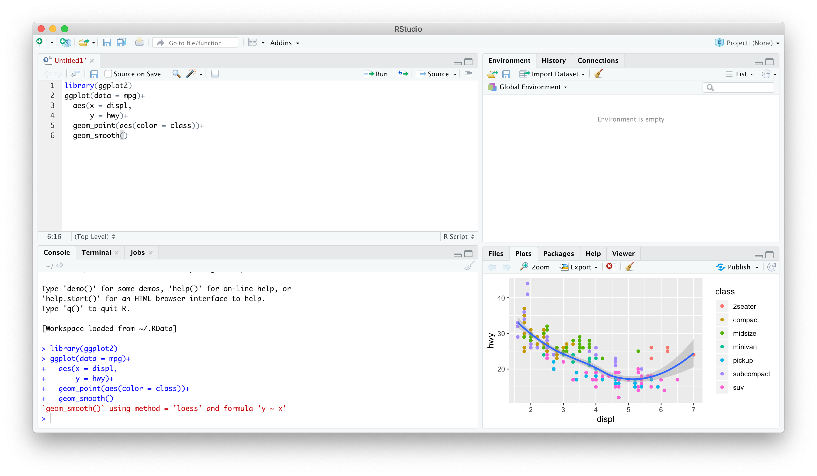
RStudio is My Text Editor of Choice
- Honestly, I write everything in R Studio’s text editor
- Syntax highlighting
- Actually can run R code, autocomplete, etc
- Can render the markdown to an output format: html, pdf, etc.
- You can write R code in other text editors, but you can’t execute them outside of R Studio (or the command line, but that’s too advanced.) Same with actually rendering your markdown to an output (pdf, html, etc)
knitr
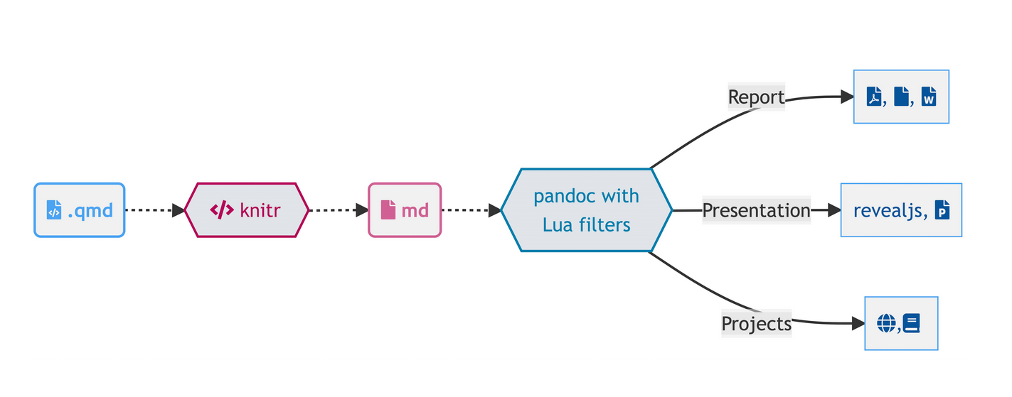
When you are ready, you “redner” your markdown and code into an output format using:
knitr1, an R package that “knits” your R code and markdown.qmdinto a.mdfile for:pandoc is a “swiss-army knife” utility that can convert between dozens of document types
All you need to do is click the
Renderbutton at the top of the text editor!
R Projects I
- A
R Projectis a way of systematically organizing yourRhistory, working directory, and related files in a single, self-contained directory - Can easily be sent to others who can reproduce your work easily
- Connects well with version control software like GitHub
- Can open multiple projects in multiple windows
R Projects I
- Projects solve all of the following problems:
- Organizing your files (data, plots, text, citations, etc)
- Having an accessible working directory (for loading and saving data, plots, etc)
- Saving and reloading your commands history and preferences
- Sending files to collaborators, so they have the same working directory as you
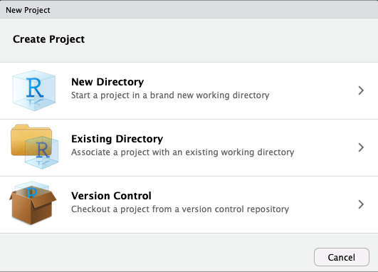
Creating an R Project I
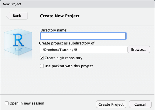
Creating an R Project II
Creating an R Project III
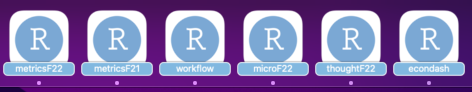
Projects
- Switch between each project (Window) on your computer (this is on a Mac)
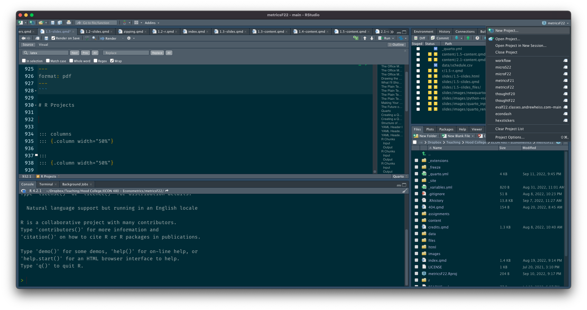
Projects
- At top right corner of RStudio
- Click the button to the right of the name to open in a new window!
Loading Others’ Projects
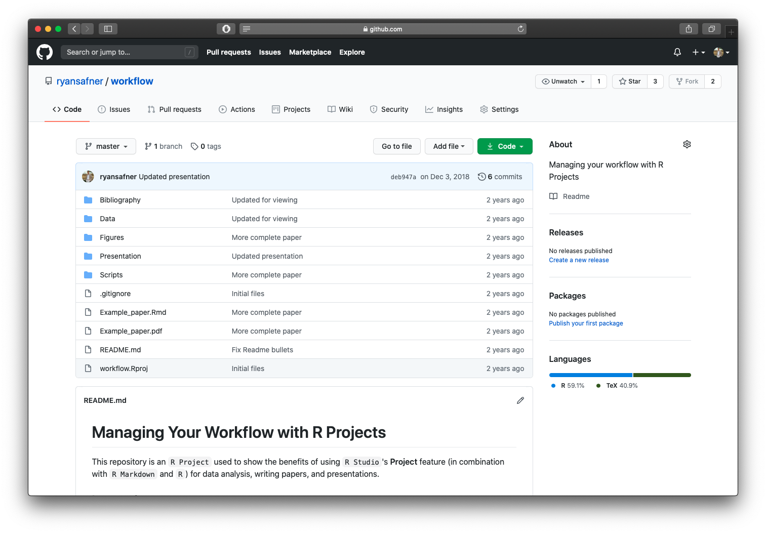
A Good File Structure
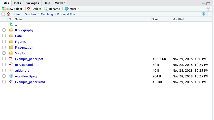
- Look through this on your own
- Read the
READMEof this repository on GitHub for instructions (automatically shows on the main page) - Look at the
example_paper.qmd- Uses data from data folder
- Uses
.Rscripts from scripts folder - Uses figures from figures folder
- Uses
bibexample.bibfrom bibliography folder
Have You Done This?
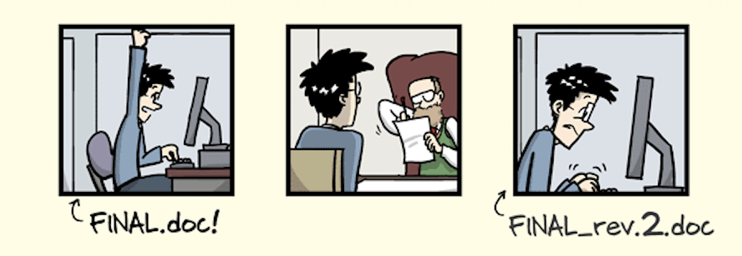
Source: PhD Comics
Have You Done This?
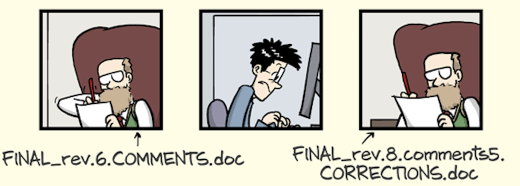
Source: PhD Comics
Have You Done This?
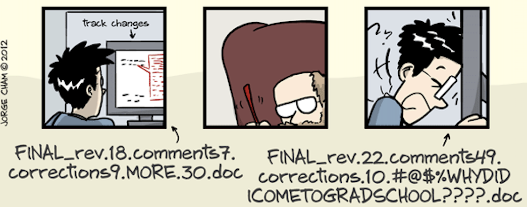
Source: PhD Comics
Do You Want to Be Able to
Keep your files backed up
Track changes
Collaborate on the same files with others
Edit files on one computer and then open and continue working on another?
The Training-Wheels Version

Register an account for free
Set up a location on your computer for the
Dropbox/folderAnything you put in this folder will sync to the cloud
- As soon as you change files, they automatically update and sync!
- Can download any of these flies from the website on any device
- Set this up on multiple computers so when you change a file on one, it updates on all the others!
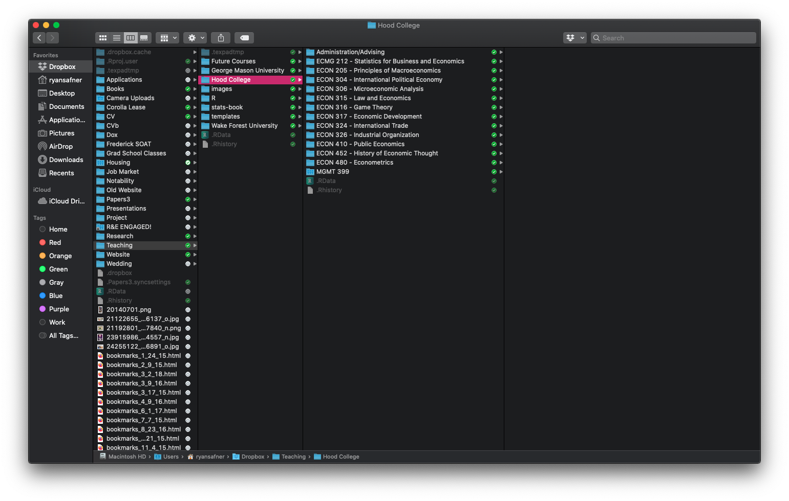
My Life Goes In Here
Smart Sync
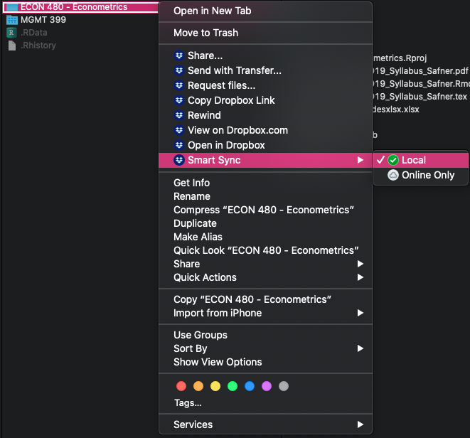
Smart Sync - keep some files online only for space
The Expert Version

Gitis an “open source distributed version control system” widely used in the software development industryTrack changes on steroids (if MS Word’s Track Changes and Dropbox had a baby)
- Organize folders/files to track (a
"repository") - Take a snapshot of all of your files (a “
commit”) with “comments” pushthese to the cloudpullchanges to (other) computers as needed
- Organize folders/files to track (a
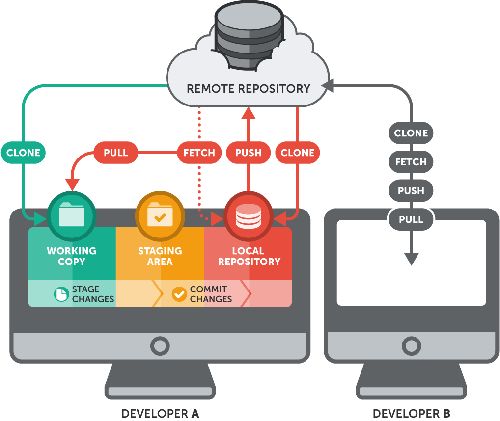
GitHubis a popular (not the only!) cloud destination for these repositories
The Expert Version
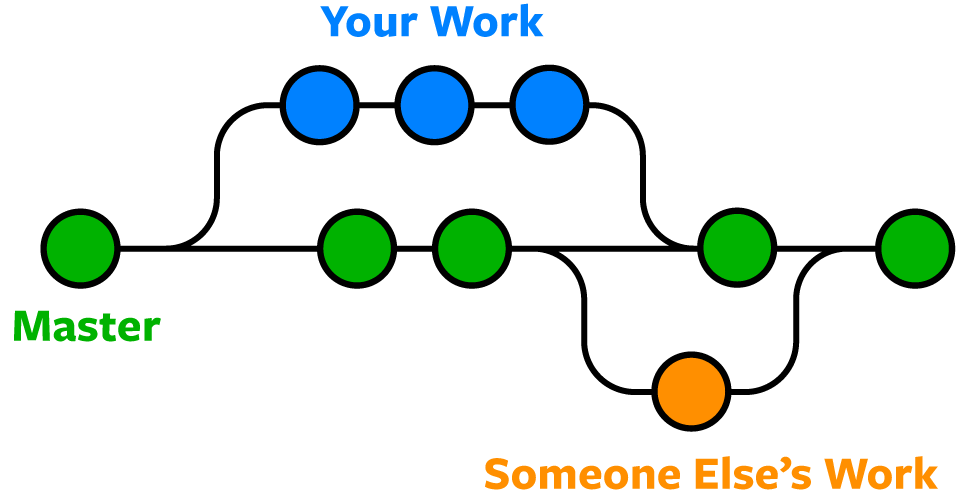
- Shows history (
versions) of files with comments- Can
forkorbranchrepository into multiple versions at once - Good for “testing” things out without destroying old versions!
revertback to original versions as needed
- Can
The Expert Version
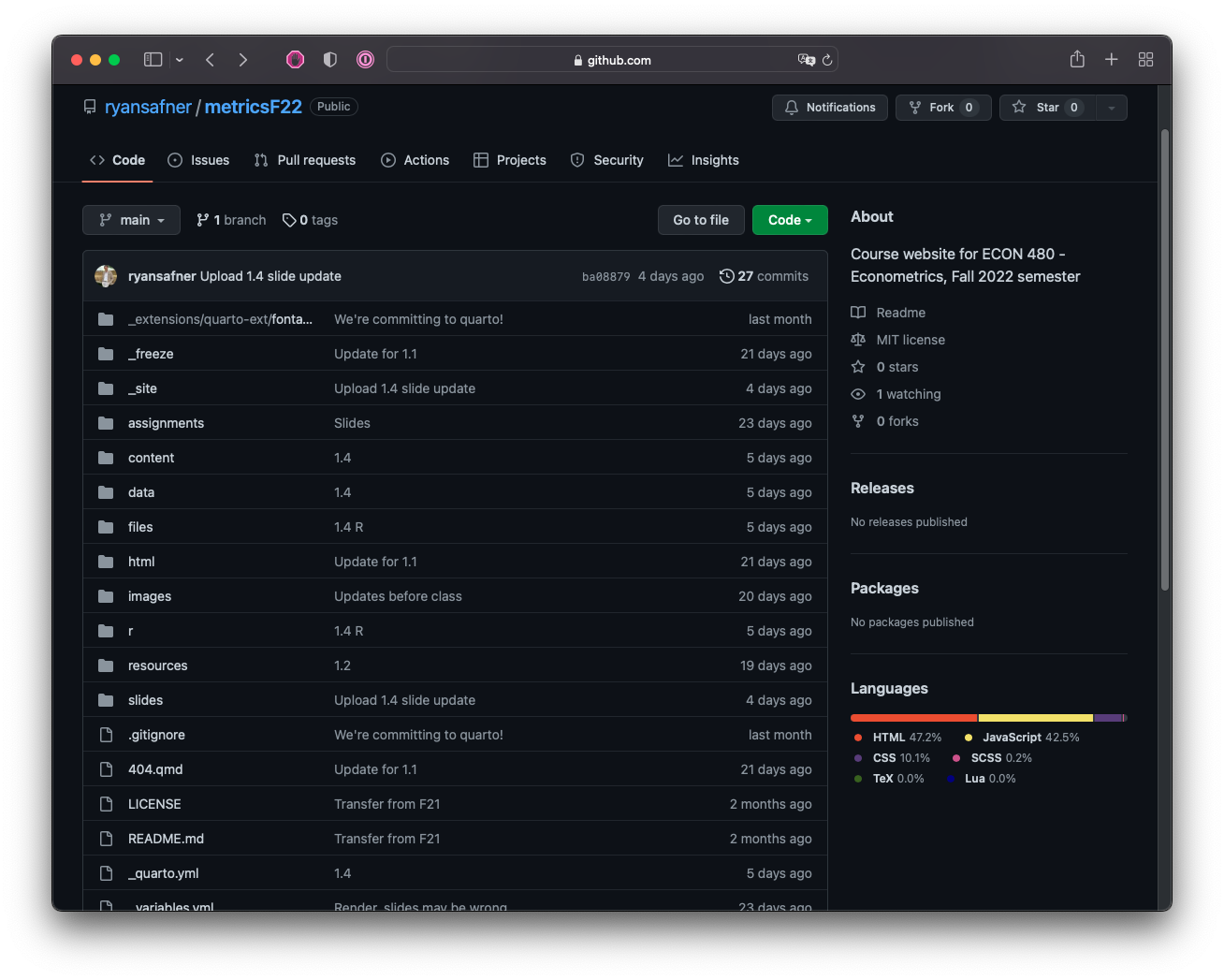
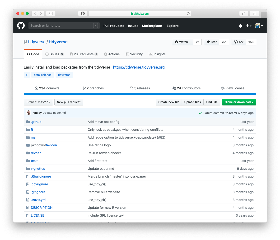
This Class on Github
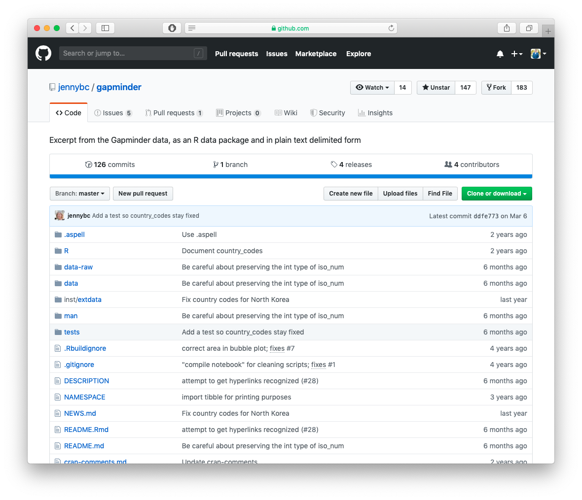
Most Packages Start on Github
Resources
- Quarto Documentation: Tutorial: Hello, Quarto
- Quarto Documentation: Tutorial: Computation
- Quarto Documentation: Tutorial: Authoring
- Quarto Documentation: Guide
- Kieran Healey’s The Plain Person’s Guide to Plain Text Social Science on managing workflow with plain text files, R, and Git
- Hadley Wickham’s (and Garrett Grolemund) R for Data Science on how to use R and R Markdown for data science work
- Jenny Bryan’s Happy Git with R on how to use git and GitHub with R as a version control system
