Experiments
- An experiment is any procedure that can (in principle) be repeated infinitely and has a well-defined set of outcomes
Example
Flip a coin 10 times.
Random Variables
A random variable (RV) takes on values that are unknown in advance, but determined by an experiment
A numerical summary of a random outcome
Example
The number of heads from 10 coin flips
Discrete Random Variables
- A discrete random variable: takes on a finite/countable set of possible values
Example
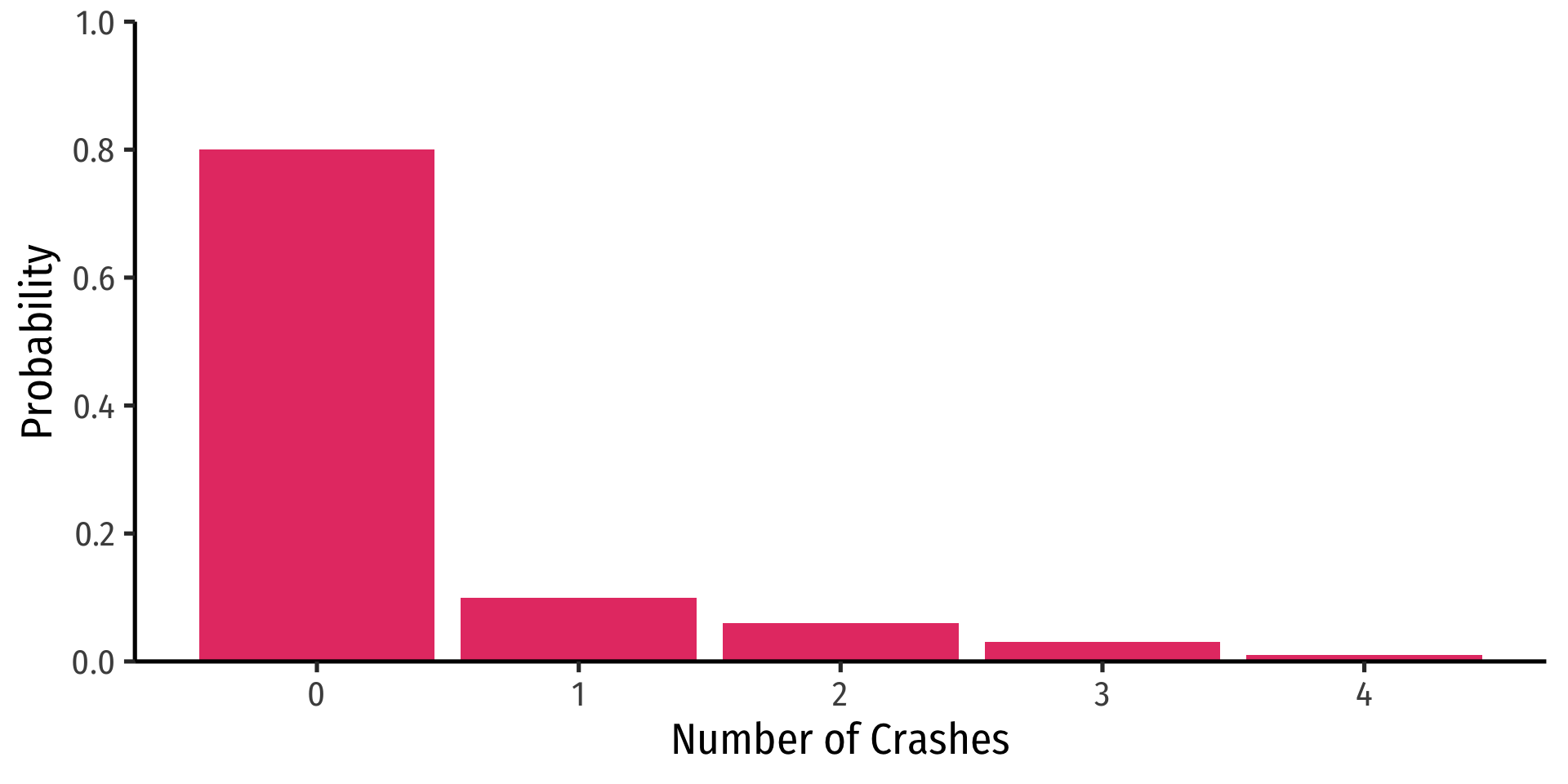
Let \(X\) be the number of times your computer crashes this semester1, \(x_i \in \{0, 1, 2, 3, 4\}\)

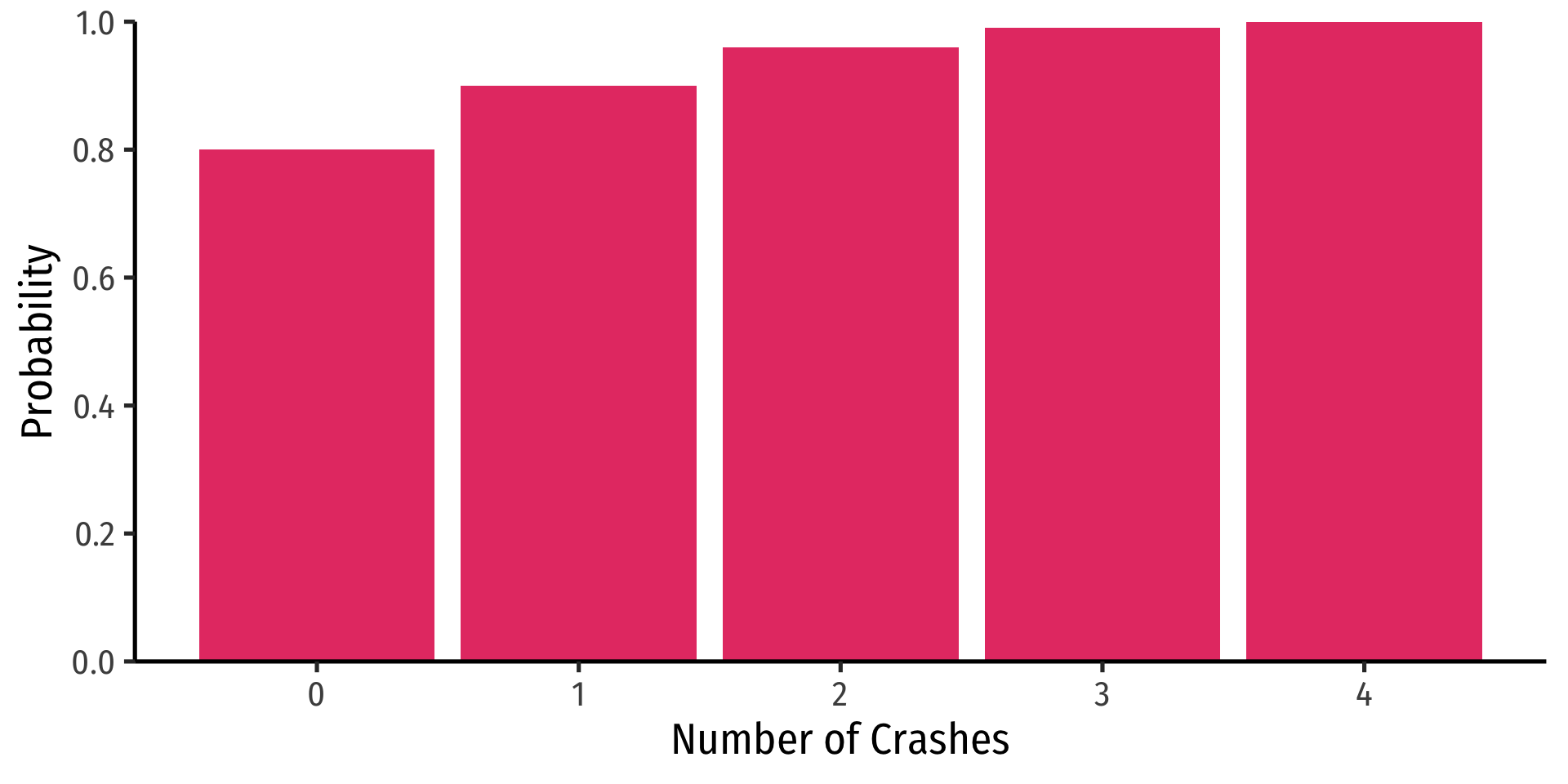
Discrete Random Variables: cdf Graph
Continuous Random Variables
Continuous random variables can take on an uncountable (infinite) number of values
So many values that the probability of any specific value is infinitely small:
\[P(X=x_i)\rightarrow 0\]
- Instead, we focus on a range of values it might take on

Continuous Random Variables: pdf I
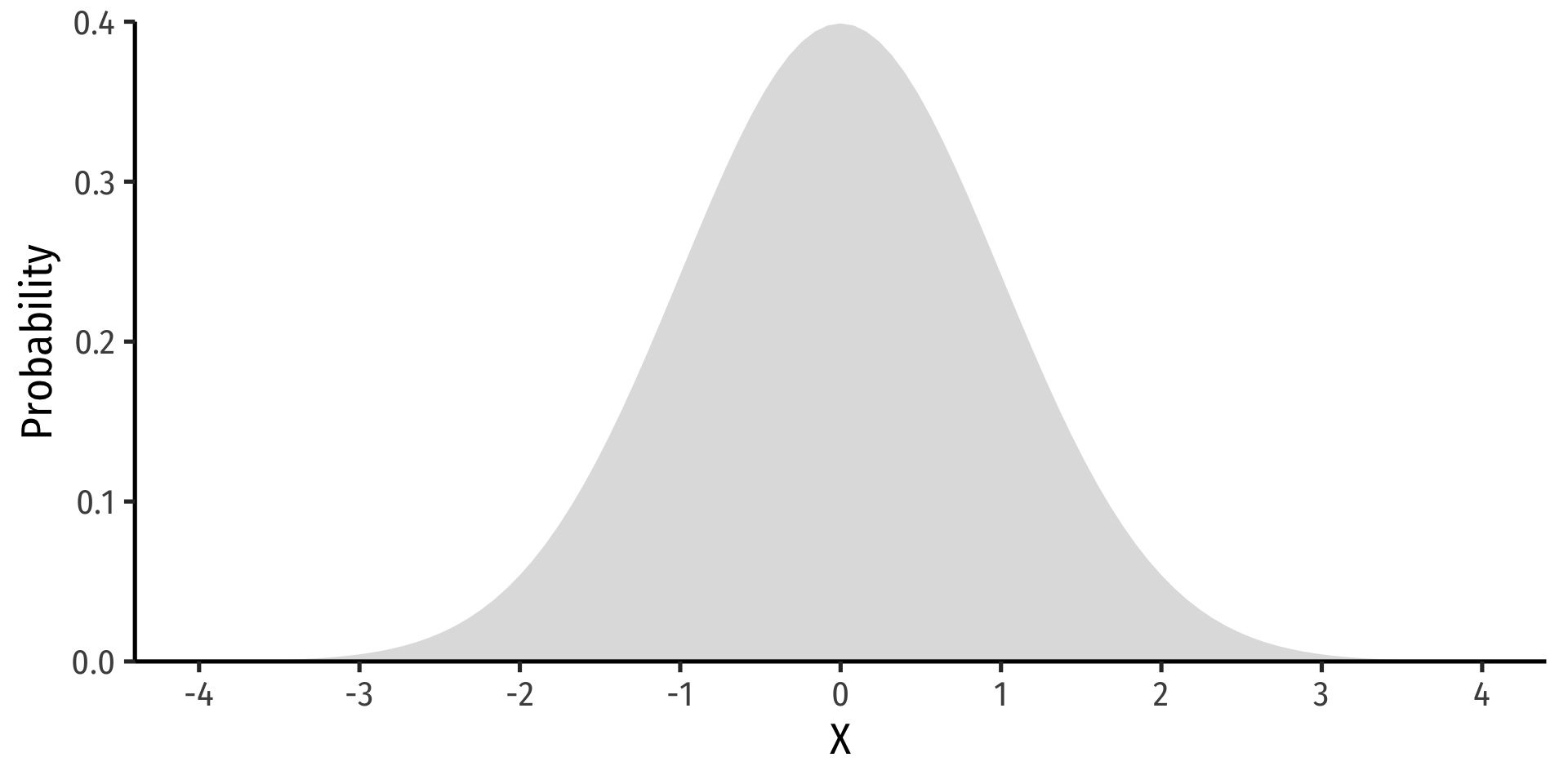
Probability density function (pdf) of a continuous variable represents the probability between two values as the area under a curve
The total area under the curve is 1
Since \(P(a)=0\) and \(P(b)=0\), \(P(a<X<b)=P(a \leq X \leq b)\)
See today’s appendix for how to graph math/stats functions in
ggplot!
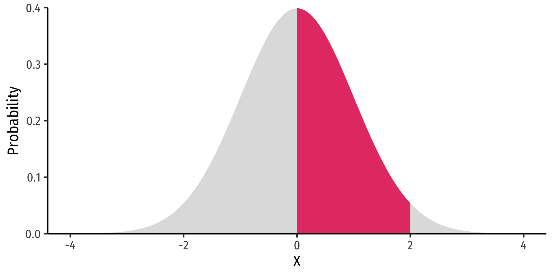
Example
\(P(0 \leq X \leq 2)\)
Continuous Random Variables: pdf II
- FYI using calculus:
\[P(a \leq X \leq b) = \int_a^b f(x) dx \]
- Complicated: software or (old fashioned!) probability tables to calculate

Example
\(P(0 \leq X \leq 2)\)
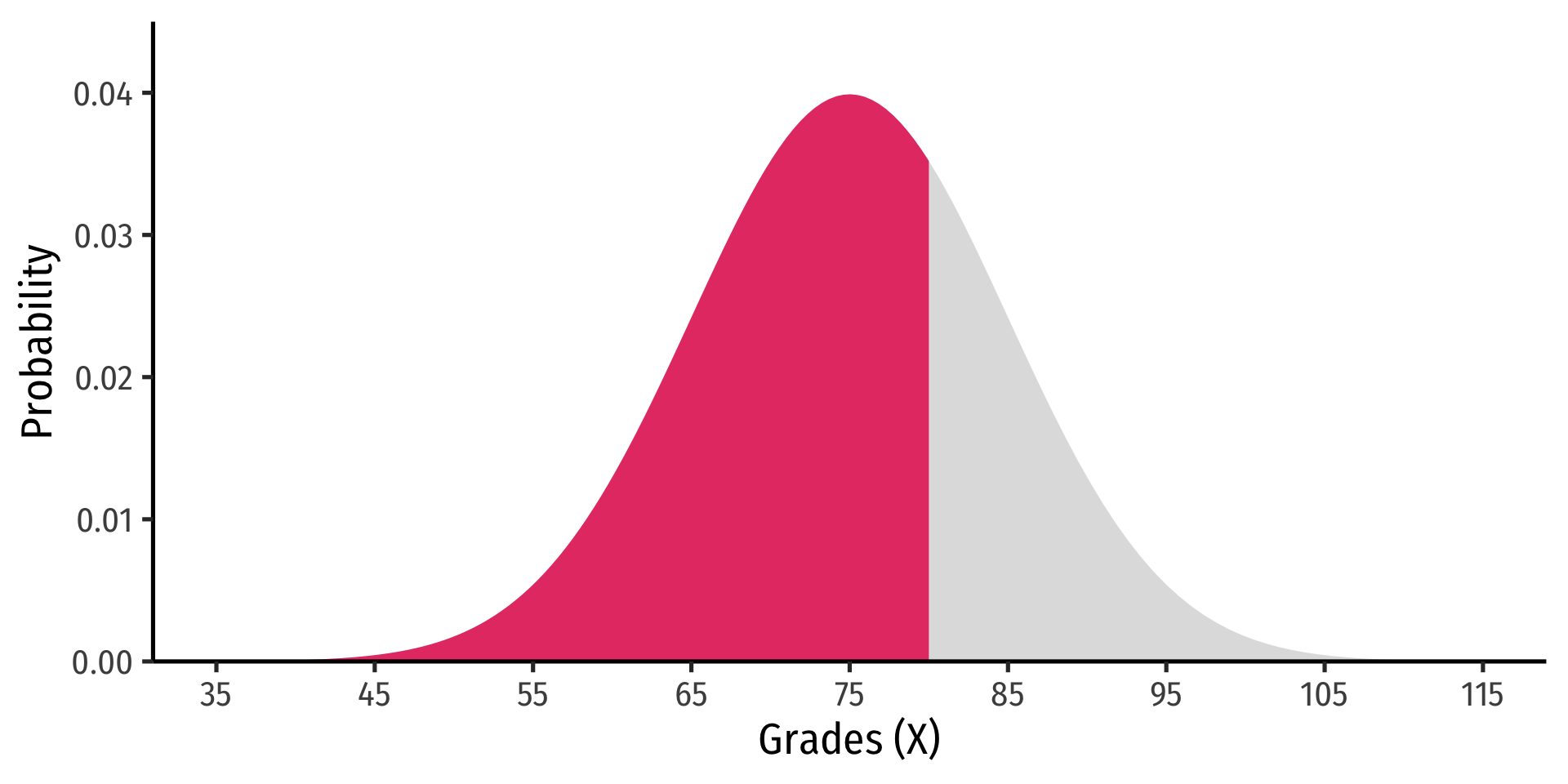
Continuous Random Variables: cdf I
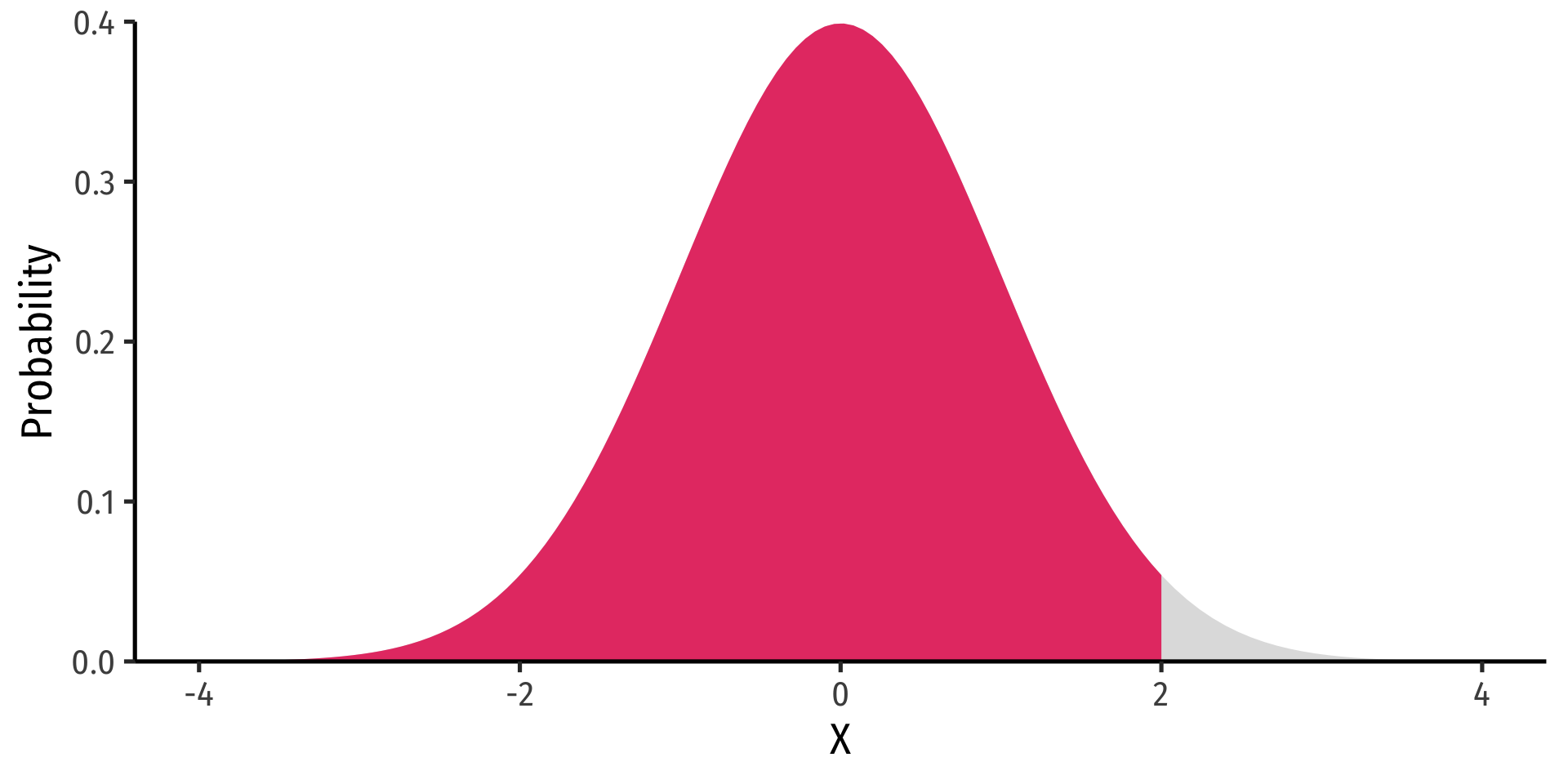
- The cumulative density function (cdf) describes the area under the pdf for all values less than or equal to (i.e. to the left of) a given value, \(k\)
\[P(X \leq k)\]
Example
\(P(X \leq 2)\)

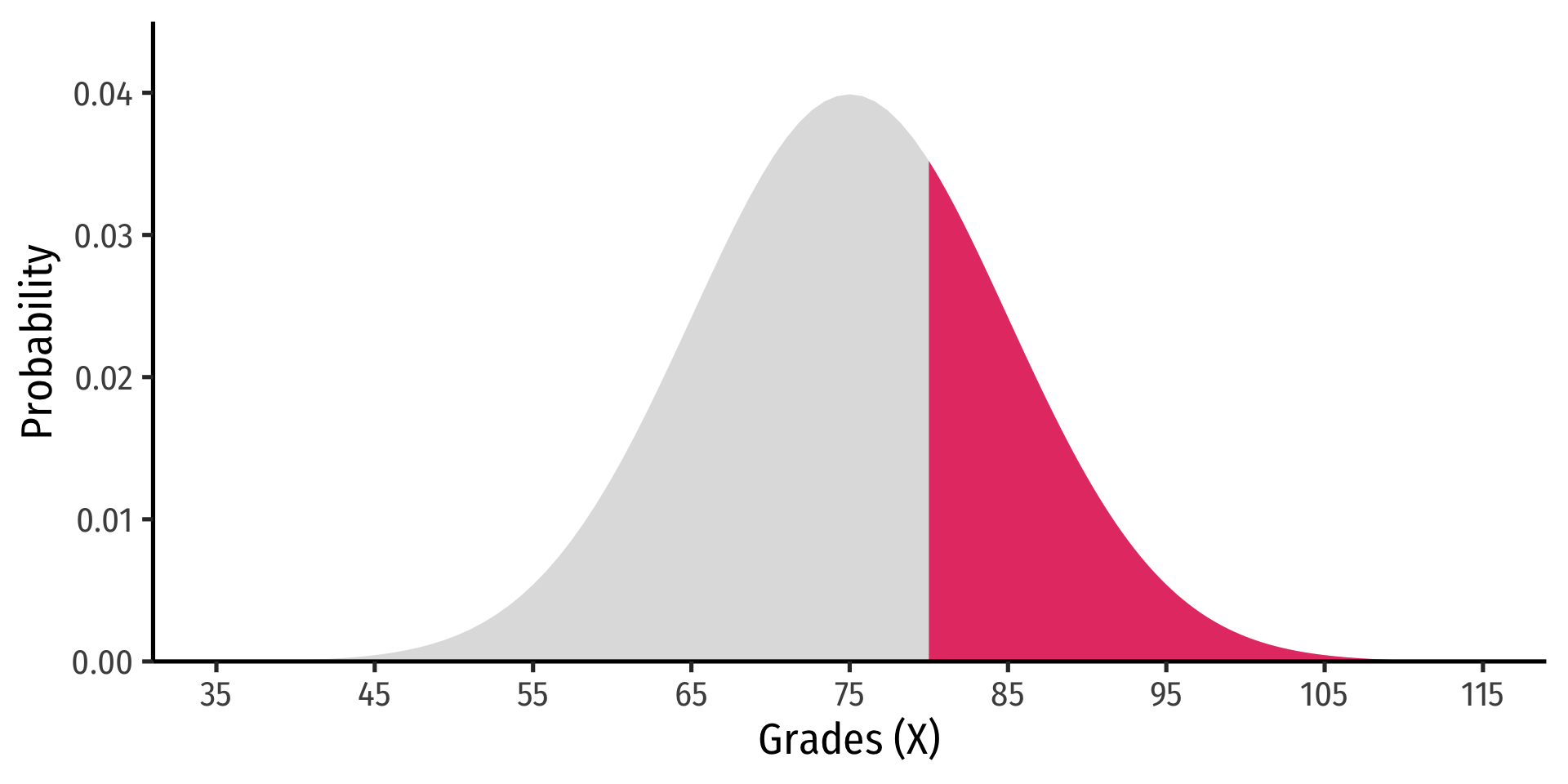
Continuous Random Variables: cdf II
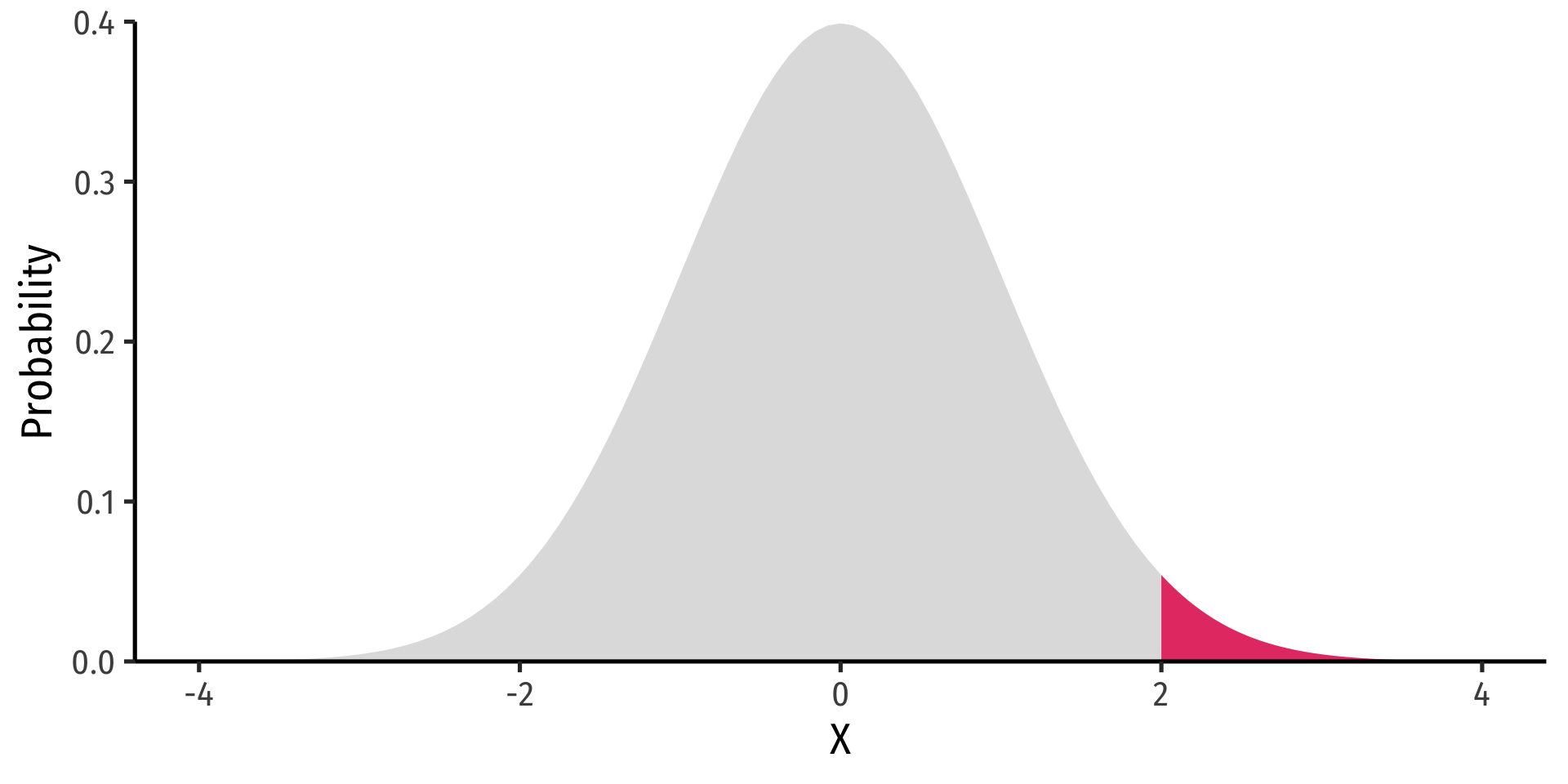
- Note: to find probability of values greater than or equal to (to the right of) a given value \(k\):
\[P(X \geq k)=1-P(X \leq k)\]
Example
\(P(X \geq 2) = 1 - P(X \leq 2)\)
\(P(X \geq 2)=\) area under the pdf curve to the right of 2
The Normal Distribution
- The Gaussian or normal distribution is the most useful type of probability distribution
\[ X \sim N(\mu,\sigma)\]
“\(X\) is distributed Normally with mean \(\mu\) and standard deviation \(\sigma\)”
Continuous, symmetric, unimodal

The Normal Distribution: pdf
- FYI: The pdf of \(X \sim N(\mu, \sigma)\) is
\[P(X=k)= \frac{1}{\sqrt{2\pi \sigma^2}}e^{-\frac{1}{2}\big(\frac{(k-\mu)}{\sigma}\big)^2}\]
- Do not try and learn this, we have software and (previously tables) to calculate pdfs and cdfs

The Standard Normal Distribution
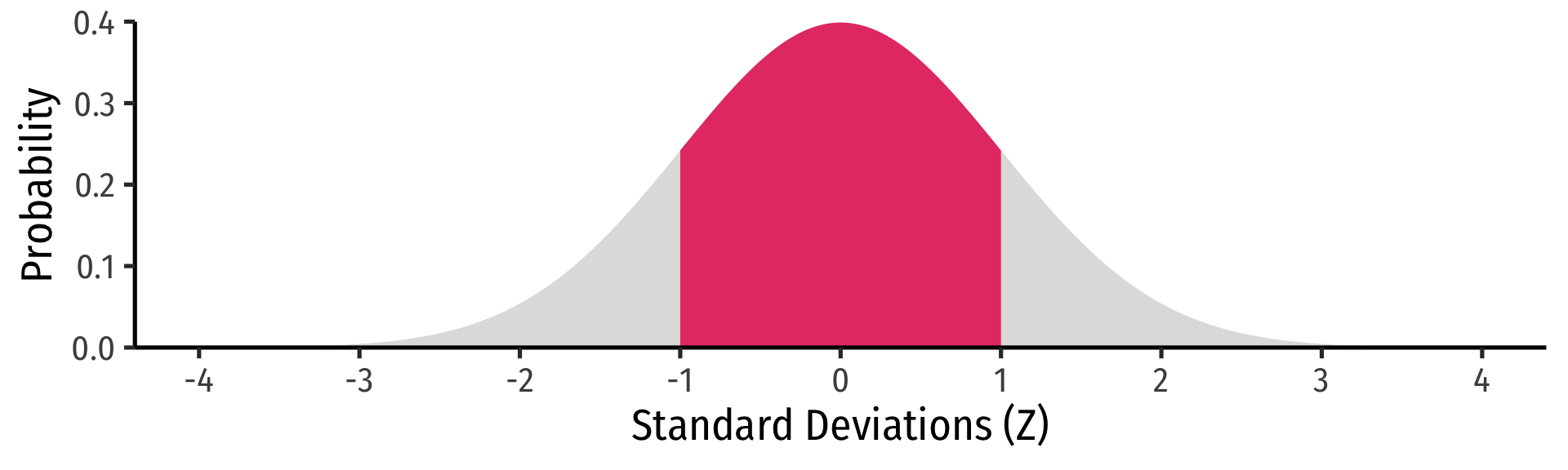
- The standard normal distribution (often referred to as \(Z\)) has mean 0 and standard deviation 1
\[Z \sim N(0,1)\]
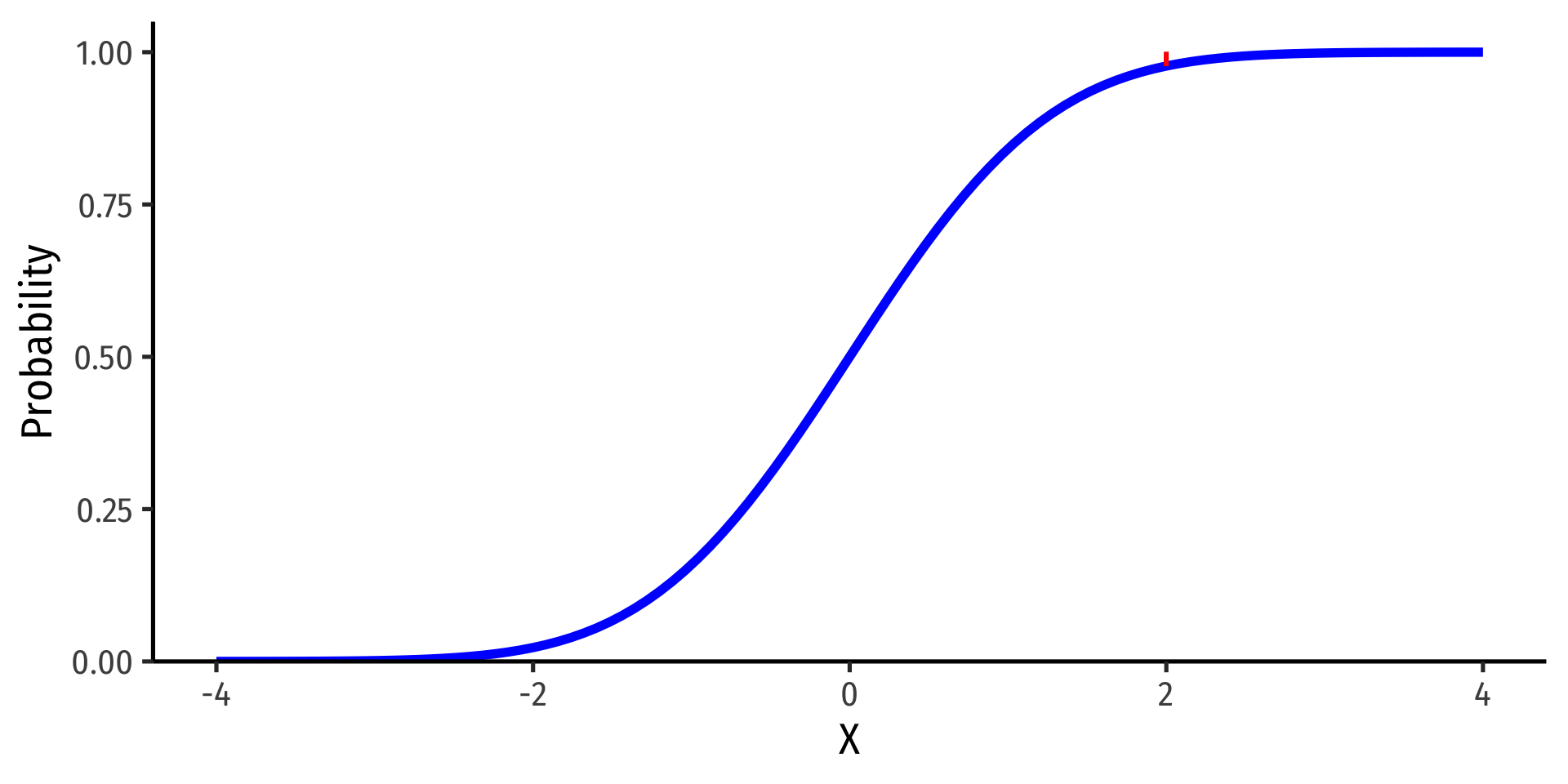
The Standard Normal cdf
- The standard normal cdf, often referred to as \(\Phi\):
\[\Phi(k)=P(Z \leq k)\]
(again, the area under the pdf curve to the left of some value \(k\))

The 68-95-99.7 Empirical Rule
- 68-95-99.7% empirical rule: for a normal distribution:

The 68-95-99.7 Empirical Rule
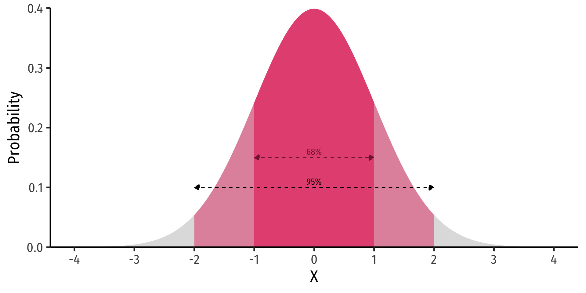
68-95-99.7% empirical rule: for a normal distribution:
\(P(\mu-1\sigma \leq X \leq \mu+1\sigma) \approx\) 68%

The 68-95-99.7 Empirical Rule
68-95-99.7% empirical rule: for a normal distribution:
\(P(\mu-1\sigma \leq X \leq \mu+1\sigma) \approx\) 68%
\(P(\mu-2\sigma \leq X \leq \mu+2\sigma) \approx\) 95%
The 68-95-99.7 Empirical Rule
68-95-99.7% empirical rule: for a normal distribution:
\(P(\mu-1\sigma \leq X \leq \mu+1\sigma) \approx\) 68%
\(P(\mu-2\sigma \leq X \leq \mu+2\sigma) \approx\) 95%
\(P(\mu-3\sigma \leq X \leq \mu+3\sigma) \approx\) 99.7%
68/95/99.7% of observations fall within 1/2/3 standard deviations of the mean

Standardizing Normal Distributions
- We can take any normal distribution (for any \(\mu, \sigma)\) and standardize it to the standard normal distribution by taking the Z-score of any value, \(x_i\):
\[Z=\frac{x_i-\mu}{\sigma}\]
Subtract any value by the distribution’s mean and divide by standard deviation
\(Z\): number of standard deviations \(x_i\) value is away from the mean

Standardizing Normal Distributions: Example II
How do we actually find the probabilities for Z−scores?
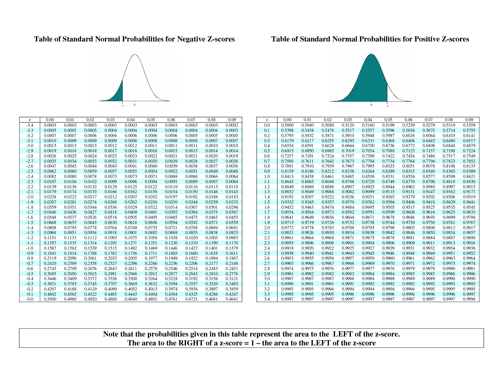
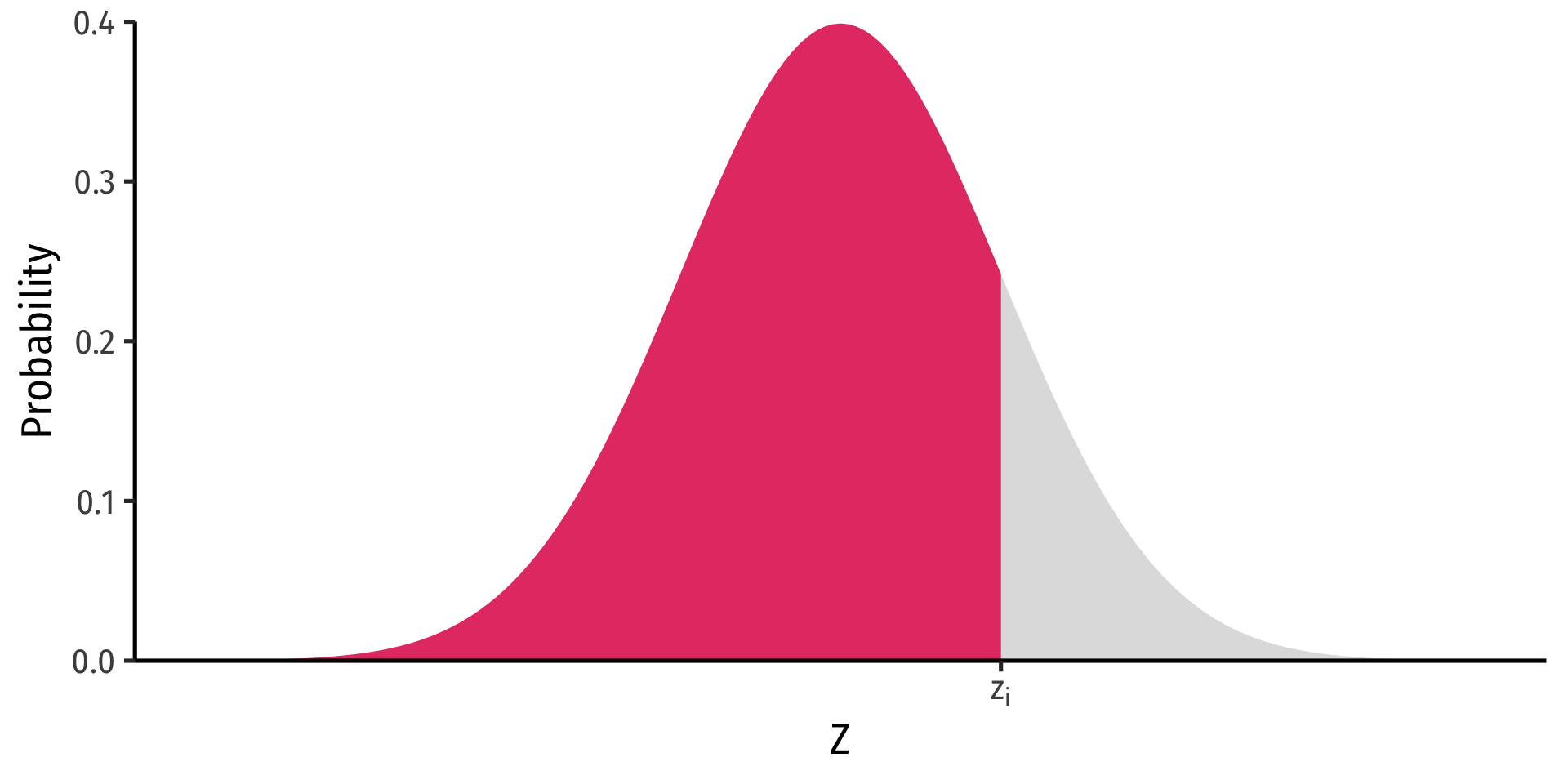
Finding Z-score Probabilities I
Probability to the left of \(z_i\)
\[P(Z \leq z_i)= \underbrace{\Phi(z_i)}_{\text{cdf of }z_i}\]
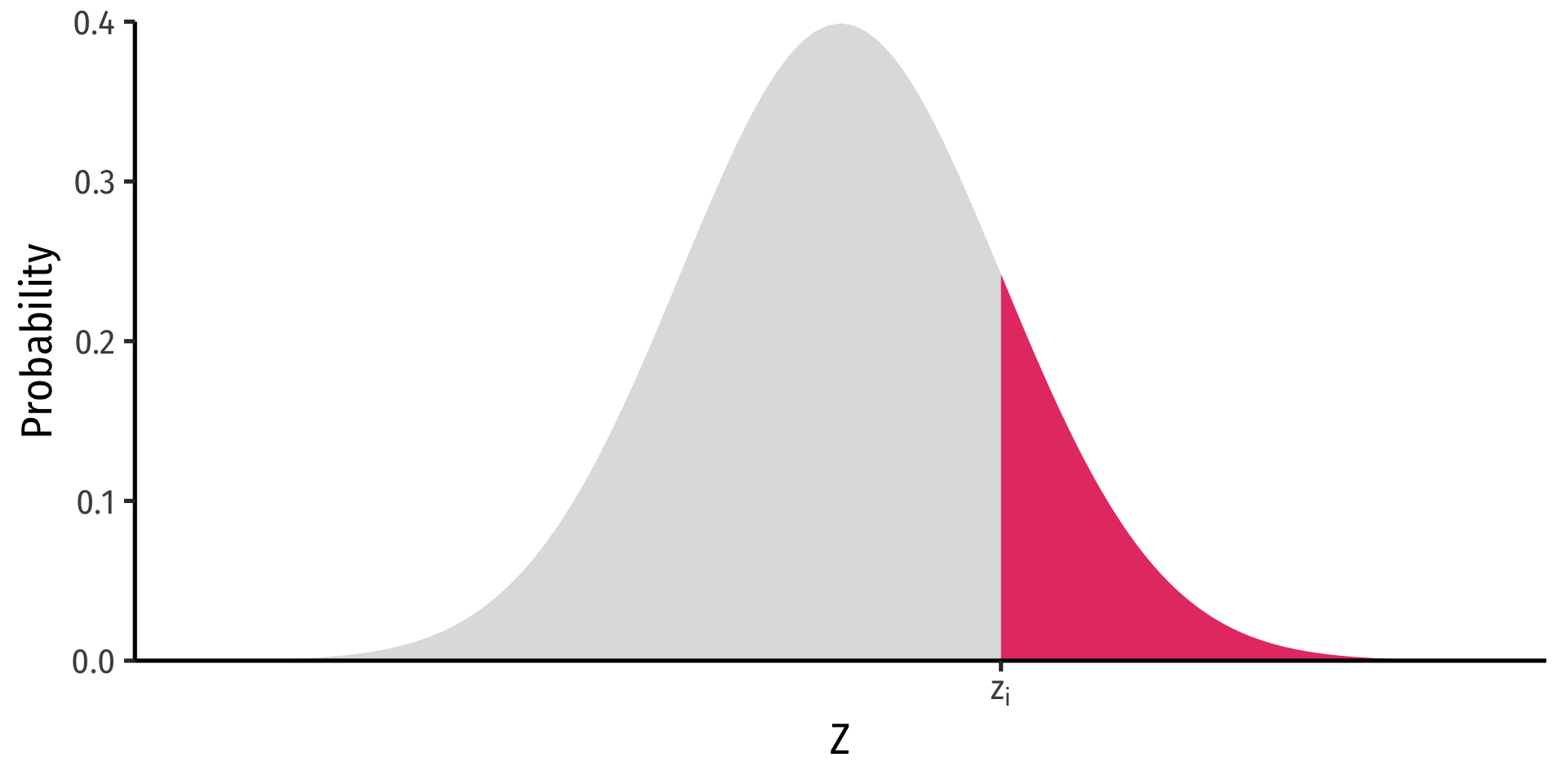
Probability to the right of \(z_i\)
\[P(Z \geq z_i)= 1-\underbrace{\Phi(z_i)}_{\text{cdf of }z_i}\]
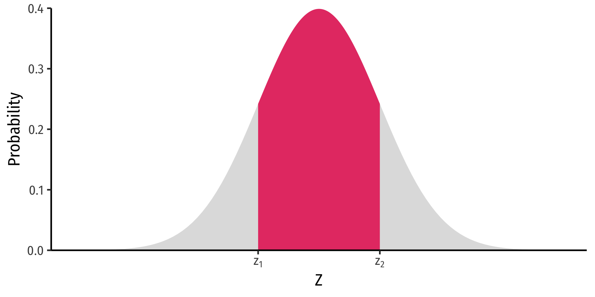
Finding Z-score Probabilities II
Probability between \(z_1\) and \(z_2\)
\[P(z_1 \geq Z \geq z_2)= \underbrace{\Phi(z_2)}_{\text{cdf of }z_2} - \underbrace{\Phi(z_1)}_{\text{cdf of }z_1}\]
Finding Z-score Probabilities III
pnorm()calculatesprobabilities with anormal distribution with arguments:x =the valuemean =the meansd =the standard deviationlower.tail =TRUEif looking at area to LEFT of valueFALSEif looking at area to RIGHT of value

Finding Z-score Probabilities IV
Finding Z-score Probabilities V
Finding Z-score Probabilities VI
Example
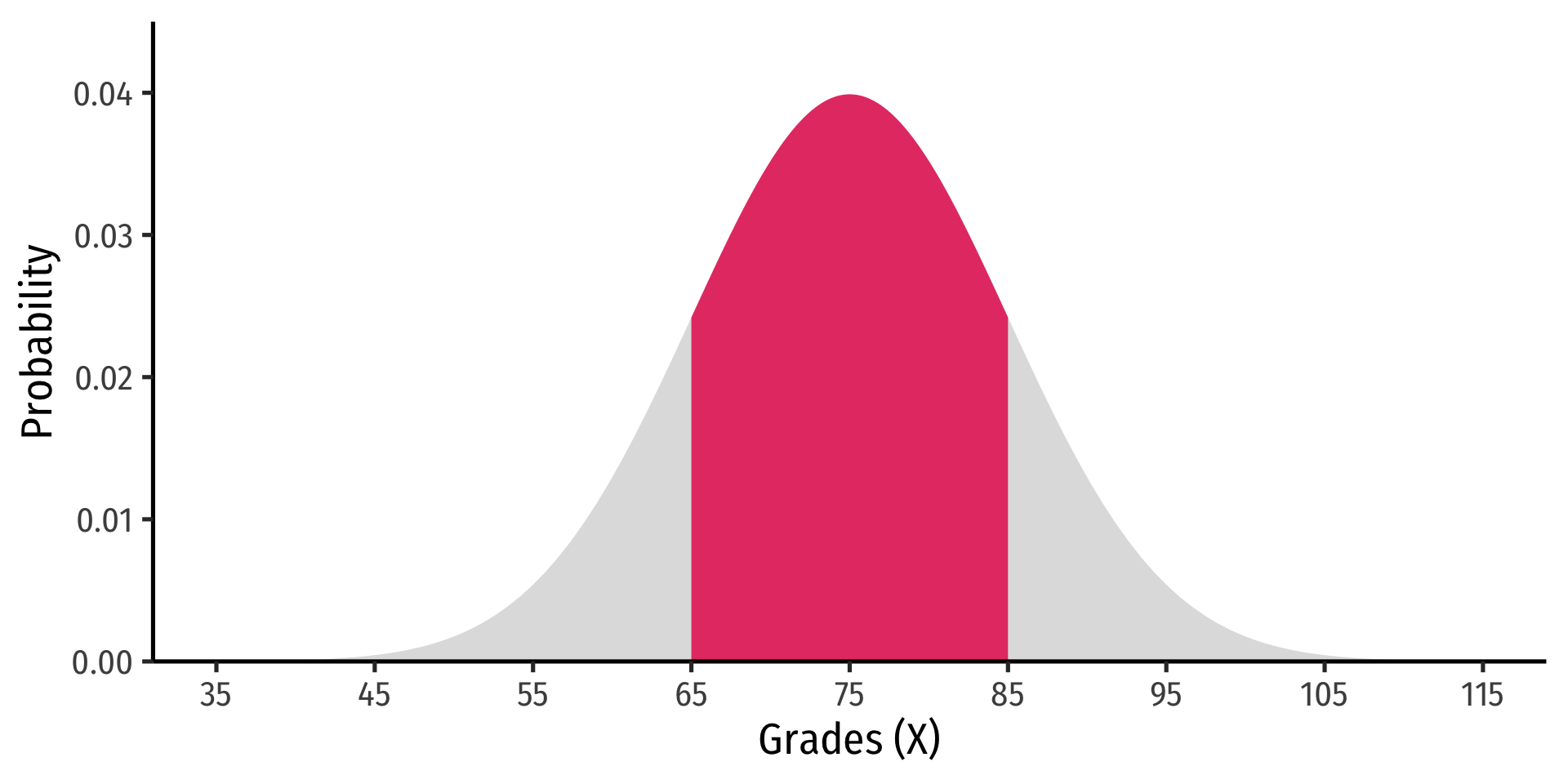
Let the distribution of grades be normal, with mean 75 and standard deviation 10.
- Probability a student gets between 65 and 85