Bivariate Data and Relationships I
- We looked at single variables for descriptive statistics
- Most uses of statistics in economics and business investigate relationships between variables
Examples
- # of police & crime rates
- healthcare spending & life expectancy
- government spending & GDP growth
- carbon dioxide emissions & temperatures
Bivariate Data and Relationships II
We will begin with bivariate data for relationships between \(X\) and \(Y\)
Immediate aim is to explore associations between variables, quantified with correlation and linear regression
Later we want to develop more sophisticated tools to argue for causation
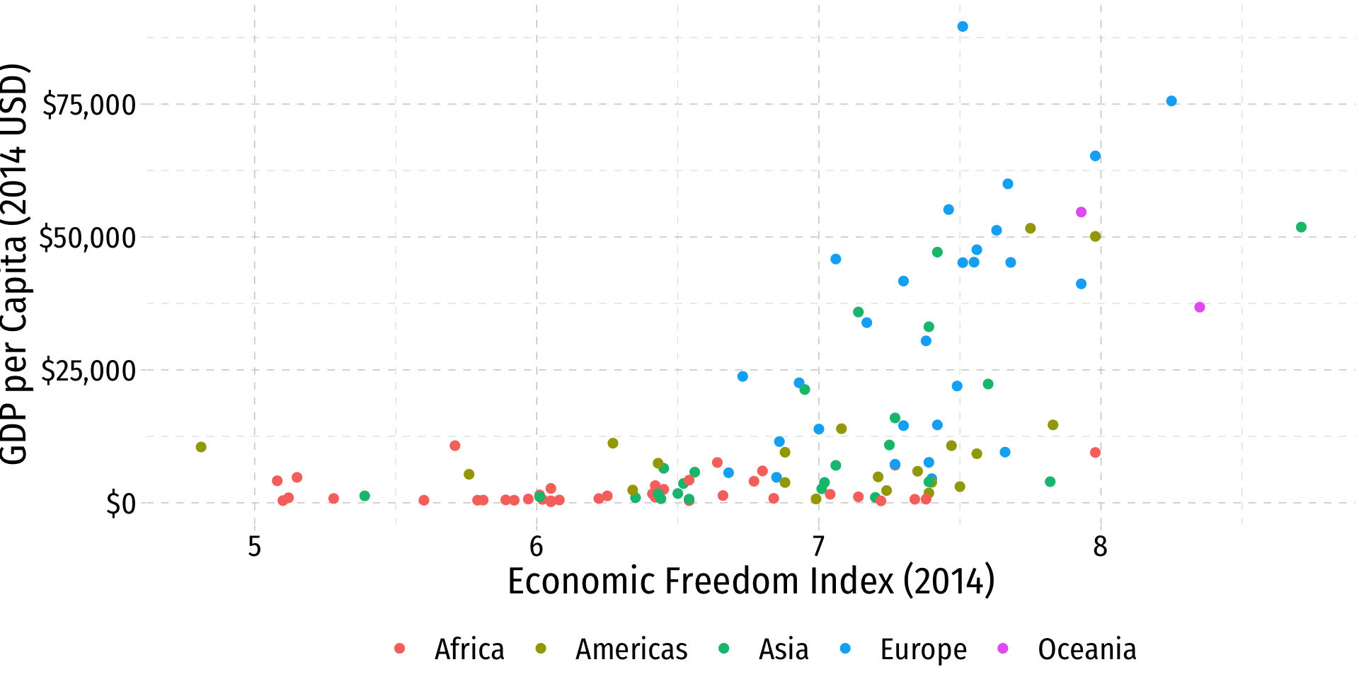
Bivariate Data: Scatterplots I
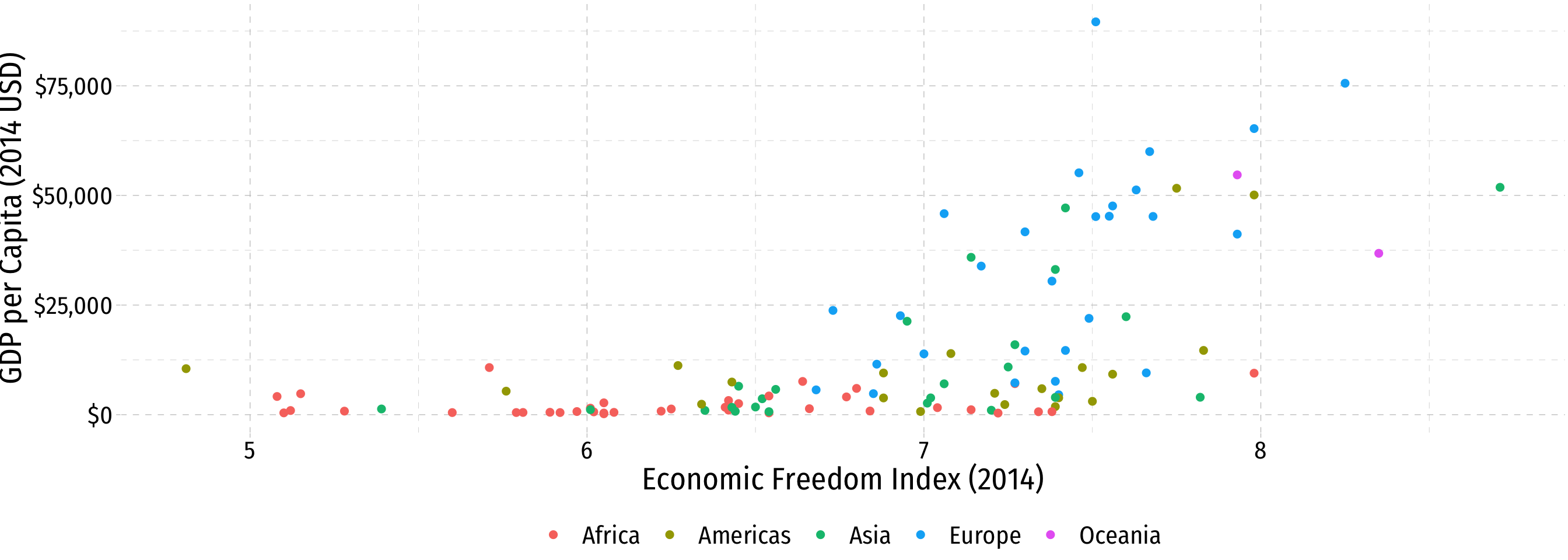
ggplot(data = econfreedom)+
  aes(x = ef,
      y = gdp)+
  geom_point(aes(color = continent),
             size = 2)+
  labs(x = "Economic Freedom Index (2014)",
       y = "GDP per Capita (2014 USD)",
       color = "")+
  scale_y_continuous(labels = scales::dollar)+
  theme_pander(base_family = "Fira Sans Condensed",
           base_size=20)+
  theme(legend.position = "bottom")
Bivariate Data: Scatterplots II
- Look for association between independent and dependent variables
Direction: is the trend positive or negative?
Form: is the trend linear, quadratic, something else, or no pattern?
Strength: is the association strong or weak?
Outliers: do any observations deviate from the trends above?
Correlation: Interpretation
- Correlation is standardized to
\[-1 \leq r \leq 1\]
Negative values \(\implies\) negative association
Positive values \(\implies\) positive association
Correlation of 0 \(\implies\) no association
As \(|r| \rightarrow 1 \implies\) the stronger the association
Correlation of \(|r|=1 \implies\) perfectly linear

Guess the Correlation!

Correlation and Endogeneity
Your Occasional Reminder: Correlation does not imply causation!
- I’ll show you the difference in a few weeks (when we can actually talk about causation)
If \(X\) and \(Y\) are strongly correlated, \(X\) can still be endogenous!
See today’s appendix page for more on Covariance and Correlation

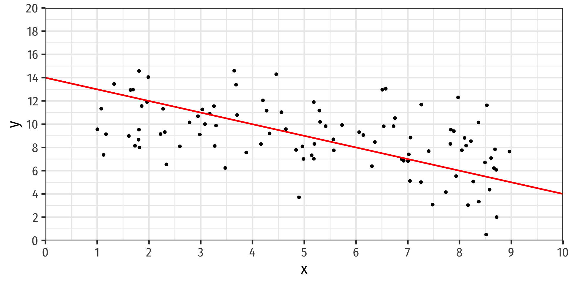
Always Plot Your Data!
Fitting a Line to Data
- If an association appears linear, we can estimate the equation of a line that would “fit” the data
\[Y = a + bX\]
- A linear equation describing a line has two parameters:
- \(a\): vertical intercept
- \(b\): slope
Fitting a Line to Data
- If an association appears linear, we can estimate the equation of a line that would “fit” the data
\[Y = a + bX\]
- A linear equation describing a line has two parameters:
- \(a\): vertical intercept
- \(b\): slope
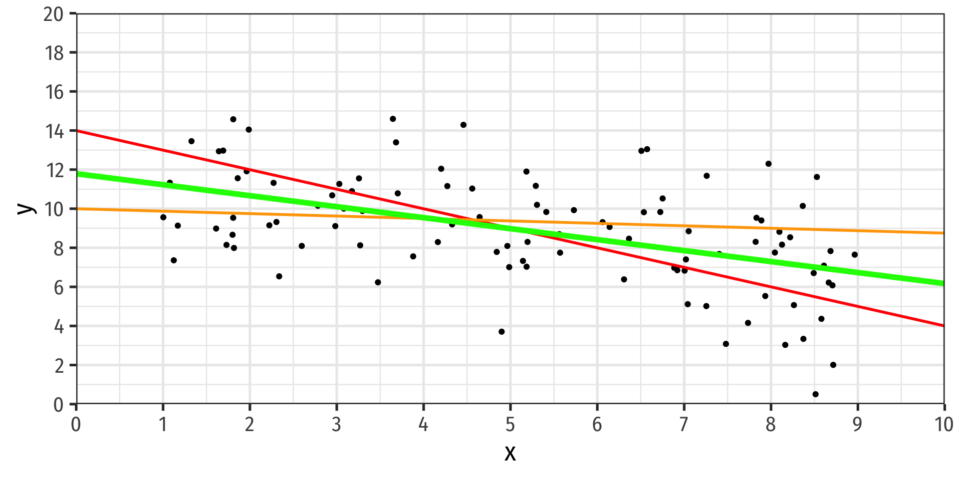
- How do we choose the equation that best fits the data?
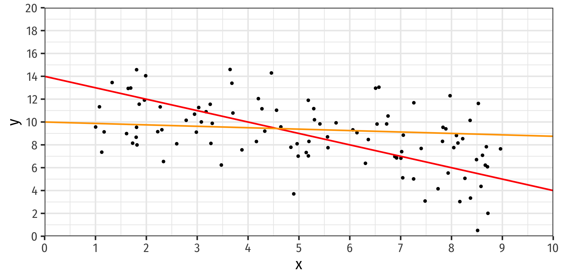
Fitting a Line to Data
- If an association appears linear, we can estimate the equation of a line that would “fit” the data
\[Y = a + bX\]
A linear equation describing a line has two parameters:
- \(a\): vertical intercept
- \(b\): slope
How do we choose the equation that best fits the data?
This process is called linear regression
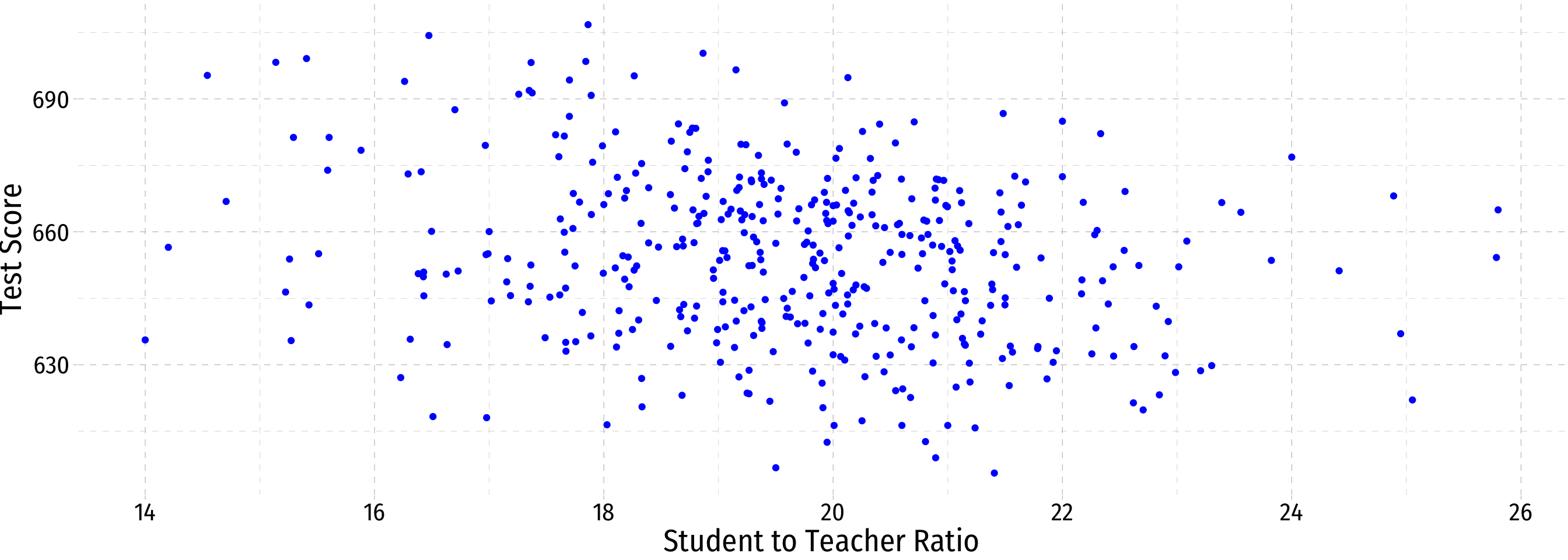
Class Size Example
Example
What is the relationship between class size and educational performance?

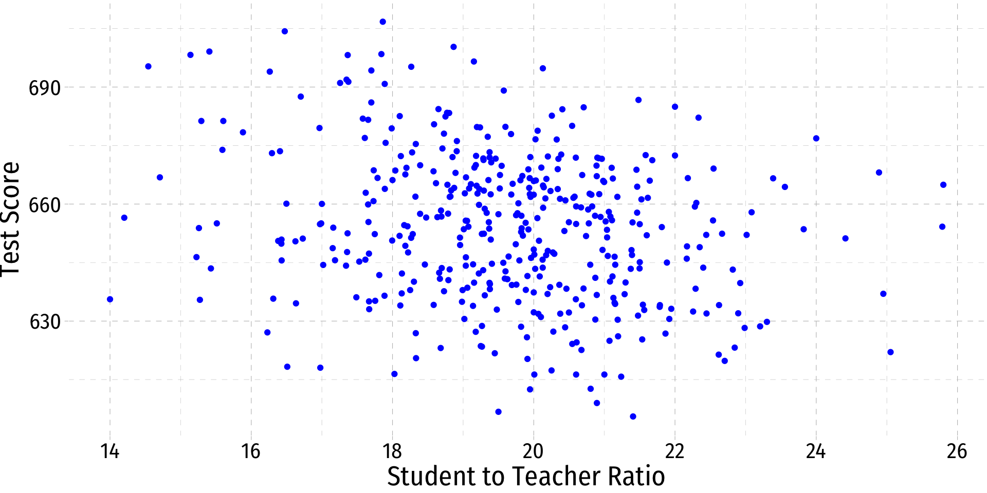
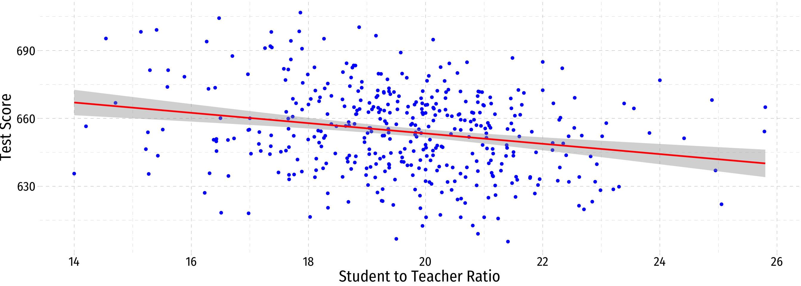
Class Size Example: Scatterplot
Class Size Example: Slope I
- If we change \((\Delta)\) the class size by an amount, what would we expect the change in test scores to be?
\[\beta = \frac{\text{change in test score}}{\text{change in class size}} = \frac{\Delta \text{test score}}{\Delta \text{class size}}\]
- If we knew \(\beta\), we could say that changing class size by 1 student will change test scores by \(\beta\)
Class Size Example: Slope II
- Rearranging:
\[\Delta \text{test score} = \beta \times \Delta \text{class size}\]
Class Size Example: Slope III
- Rearranging:
\[\Delta \text{test score} = \beta \times \Delta \text{class size}\]
- Suppose \(\beta=-0.6\). If we shrank class size by 2 students, our model predicts:
\[\begin{align*} \Delta \text{test score} &= -2 \times \beta\\ \Delta \text{test score} &= -2 \times -0.6\\ \Delta \text{test score}&= 1.2 \\ \end{align*}\]
Test scores would improve by 1.2 points, on average.
Class Size Example: Slope and Average Effect
\[\text{test score} = \beta_0 + \beta_{1} \times \text{class size}\]
The line relating class size and test scores has the above equation
\(\beta_0\) is the vertical-intercept, test score where class size is 0
\(\beta_{1}\) is the slope of the regression line
This relationship only holds on average for all districts in the population, individual districts are also affected by other factors
Class Size Example: Marginal Effect
- To get an equation that holds for each district, we need to include other factors
\[\text{test score} = \beta_0 + \beta_1 \text{class size}+\text{other factors}\]
For now, we will ignore these until Unit III
Thus, \(\beta_0 + \beta_1 \text{class size}\) gives the average effect of class sizes on scores
Later, we will want to estimate the marginal effect (causal effect) of each factor on an individual district’s test score, holding all other factors constant
The Population Regression Model
How do we draw a line through the scatterplot? We do not know the “true” \(\beta_0\) or \(\beta_1\)
We do have data from a sample of class sizes and test scores
So the real question is, how can we estimate \(\beta_0\) and \(\beta_1\)?

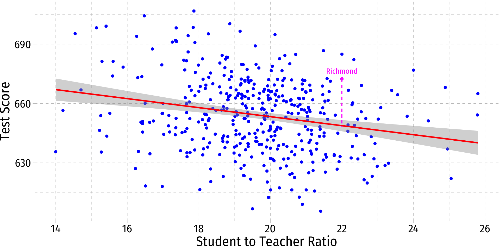
Actual, Predicted, and Residual Values
- With a simple linear regression model, for each associated \(X\) value, we have
- The observed (or actual) values of \(\color{#0047AB}{Y_i}\)

Actual, Predicted, and Residual Values
- With a simple linear regression model, for each associated \(X\) value, we have
- The observed (or actual) values of \(\color{#0047AB}{Y_i}\)
- Predicted (or fitted) values, \(\color{#047806}{\hat{Y}_i}\)
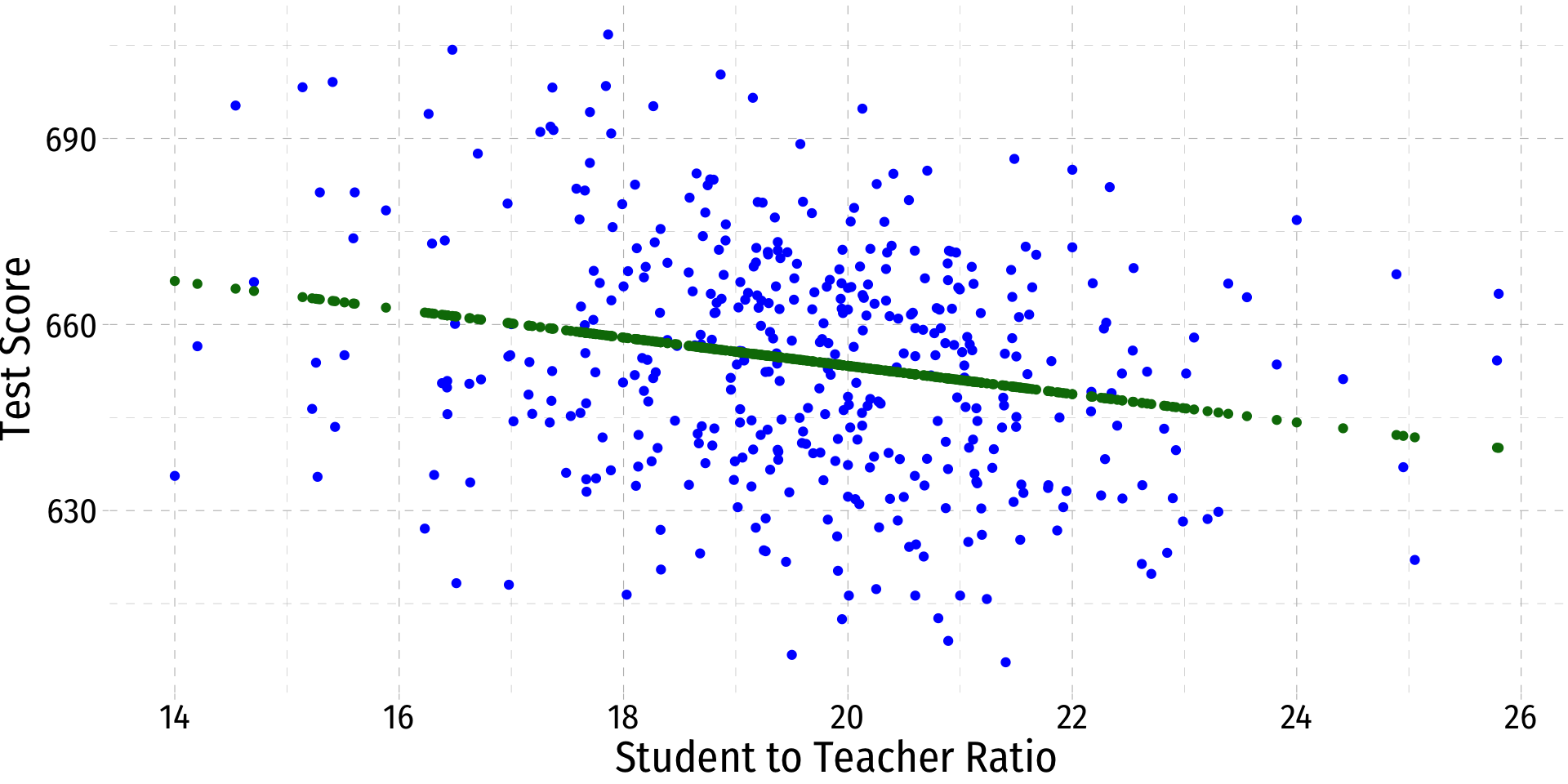
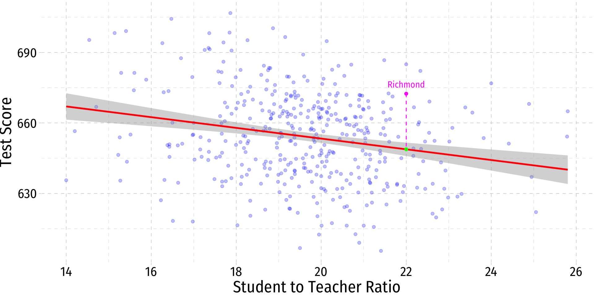
Actual, Predicted, and Residual Values
- With a simple linear regression model, for each associated \(X\) value, we have
- The observed (or actual) values of \(\color{#0047AB}{Y_i}\)
- Predicted (or fitted) values, \(\color{#047806}{\hat{Y}_i}\)
- The residual (or error), \(\color{#D7250E}{\hat{u}_i}=\color{#0047AB}{Y_i}-\color{#047806}{\hat{Y}_i}\) … the difference between predicted and observed values
\[\begin{align*} \color{#0047AB}{Y_i} &= \color{#047806}{\hat{Y}_i} + \color{#D7250E}{\hat{u}_i} \\ \color{#0047AB}{\text{Observed}_i} &= \color{#047806}{\text{Model}_i} + \color{#D7250E}{\text{Error}_i} \\ \end{align*}\]
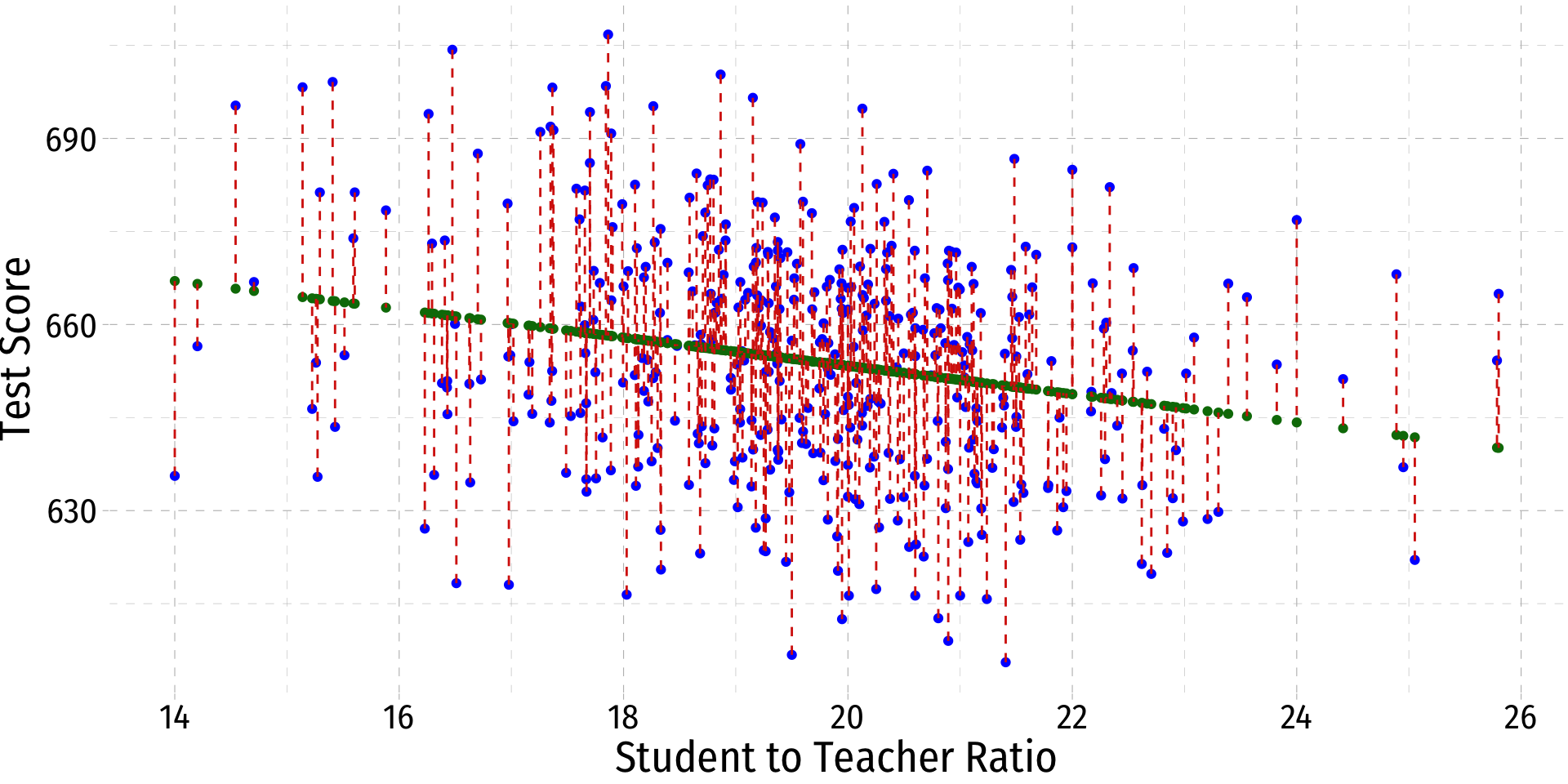
Deriving OLS Estimators
- Take the residuals \(\color{#D7250E}{\hat{u}_i}\) and square them (why)?
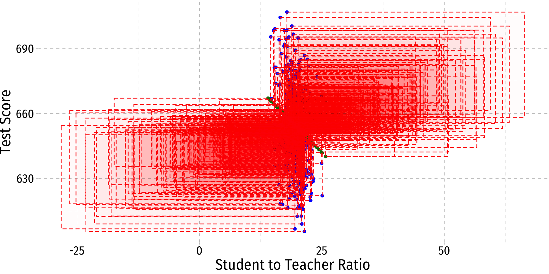
Deriving OLS Estimators
Take the residuals \(\color{#D7250E}{\hat{u}_i}\) and square them (why)?
The regression line minimizes the sum of the squared residuals (SSR)
\[SSR = \sum^n_{i=1} \color{#D7250E}{\hat{u}_i}^2\]

Class Size Scatterplot (Again)
- There is some true (unknown) population relationship:
\[\text{test score}_i=\beta_0+\beta_1 str_i\]
- \(\beta_1=\frac{\Delta \text{test score}}{\Delta \text{str}}= ??\)
Class Size Scatterplot with Regression Line
Tidy Regression with broom

The
broompackage allows us to work with regression objects as tidiertibblesSeveral useful commands:
| Command | Does |
|---|---|
tidy() |
Create tibble of regression coefficients & stats |
glance() |
Create tibble of regression fit statistics |
augment() |
Create tibble of data with regression-based variables |
Class Size Regression: An Example Data Point III
Making Predictions In R, Manually II
- Of course we could do it ourselves…
[1] -2.279808