...1 <dbl> | Country <chr> | ISO <chr> | ef <dbl> | gdp <dbl> | |
|---|---|---|---|---|---|
| 1 | Albania | ALB | 7.40 | 4543.0880 | |
| 2 | Algeria | DZA | 5.15 | 4784.1943 | |
| 3 | Angola | AGO | 5.08 | 4153.1463 | |
| 4 | Argentina | ARG | 4.81 | 10501.6603 | |
| 5 | Australia | AUS | 7.93 | 54688.4459 | |
| 6 | Austria | AUT | 7.56 | 47603.7968 | |
| 7 | Bahrain | BHR | 7.60 | 22347.9708 | |
| 8 | Bangladesh | BGD | 6.35 | 972.8807 | |
| 9 | Belgium | BEL | 7.51 | 45181.4382 | |
| 10 | Benin | BEN | 6.22 | 804.7240 |
2.3 — Simple Linear Regression
ECON 480 • Econometrics • Fall 2022
Dr. Ryan Safner
Associate Professor of Economics
safner@hood.edu
ryansafner/metricsF22
metricsF22.classes.ryansafner.com
Contents
Exploring Relationships
Bivariate Data and Relationships I
- We looked at single variables for descriptive statistics
- Most uses of statistics in economics and business investigate relationships between variables
Examples
- # of police & crime rates
- healthcare spending & life expectancy
- government spending & GDP growth
- carbon dioxide emissions & temperatures

Bivariate Data and Relationships II
We will begin with bivariate data for relationships between X and Y
Immediate aim is to explore associations between variables, quantified with correlation and linear regression
Later we want to develop more sophisticated tools to argue for causation
Bivariate Data: Spreadsheets I
- Rows are individual observations (countries)
- Columns are variables on all individuals
Bivariate Data: Spreadsheets II
Rows: 112
Columns: 6
$ ...1      <dbl> 1, 2, 3, 4, 5, 6, 7, 8, 9, 10, 11, 12, 13, 14, 15, 16, 17, 1…
$ Country   <chr> "Albania", "Algeria", "Angola", "Argentina", "Australia", "A…
$ ISO       <chr> "ALB", "DZA", "AGO", "ARG", "AUS", "AUT", "BHR", "BGD", "BEL…
$ ef        <dbl> 7.40, 5.15, 5.08, 4.81, 7.93, 7.56, 7.60, 6.35, 7.51, 6.22, …
$ gdp       <dbl> 4543.0880, 4784.1943, 4153.1463, 10501.6603, 54688.4459, 476…
$ continent <chr> "Europe", "Africa", "Africa", "Americas", "Oceania", "Europe…
Bivariate Data: Spreadsheets III
| ABCDEFGHIJ0123456789 |
Variable <chr> | Obs <dbl> | Min <dbl> | Q1 <dbl> | Median <dbl> | |
|---|---|---|---|---|---|
| ef | 112 | 4.81 | 6.42 | 7.0 | |
| gdp | 112 | 206.71 | 1307.46 | 5123.3 |
2 rows | 1-5 of 9 columns
Bivariate Data: Scatterplots I
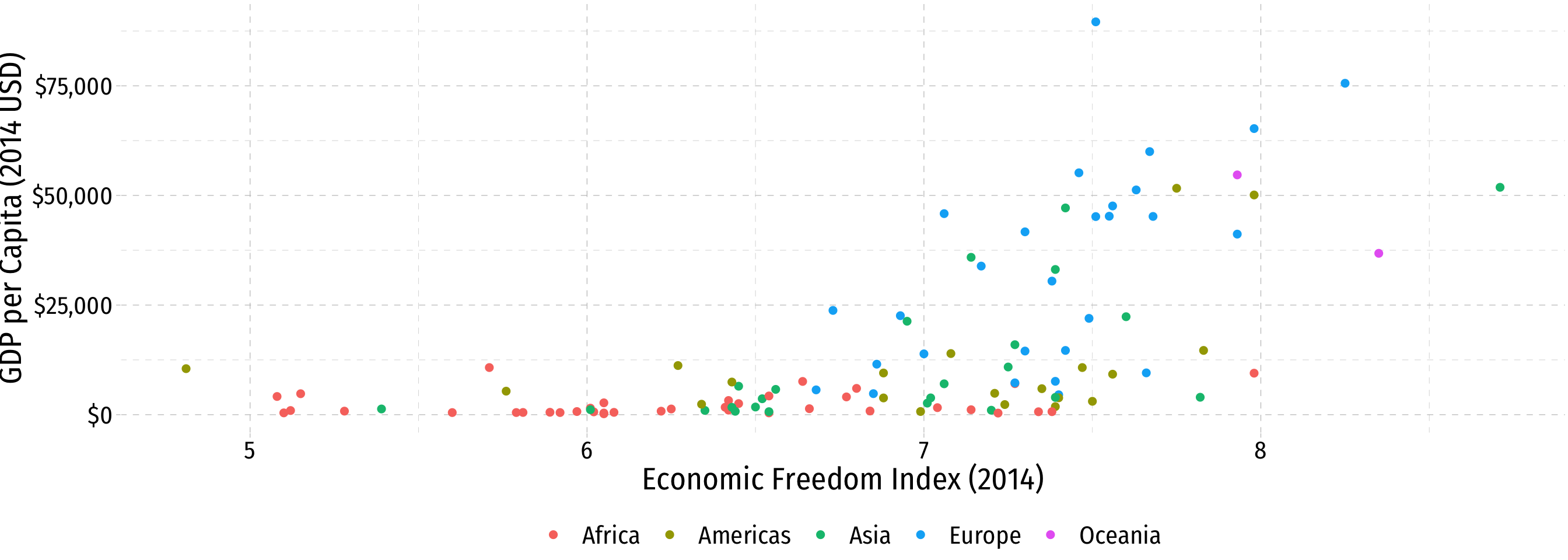
ggplot(data = econfreedom)+
  aes(x = ef,
      y = gdp)+
  geom_point(aes(color = continent),
             size = 2)+
  labs(x = "Economic Freedom Index (2014)",
       y = "GDP per Capita (2014 USD)",
       color = "")+
  scale_y_continuous(labels = scales::dollar)+
  theme_pander(base_family = "Fira Sans Condensed",
           base_size=20)+
  theme(legend.position = "bottom")
Bivariate Data: Scatterplots II
- Look for association between independent and dependent variables
Direction: is the trend positive or negative?
Form: is the trend linear, quadratic, something else, or no pattern?
Strength: is the association strong or weak?
Outliers: do any observations deviate from the trends above?
Quantifying Relationships
Covariance
- For any two variables, we can measure their sample covariance, cov(X,Y) or sX,Y to quantify how they vary together1
sX,Y=E[(X−ˉX)(Y−ˉY)]
- Intuition: if xi is above the mean of X, would we expect the associated yi:
- to be above the mean of Y also (X and Y covary positively)
- to be below the mean of Y (X and Y covary negatively)
- Covariance is a common measure, but the units are meaningless, thus we rarely need to use it so don’t worry about learning the formula
Covariance, in R
8923 what, exactly?
Correlation
- Better to standardize covariance into a more intuitive concept: correlation, rX,Y ∈[−1,1]
rX,Y=sX,YsXsY=cov(X,Y)sd(X)sd(Y)
- Simply weight covariance by the product of the standard deviations of X and Y
- Alternatively, take the average1 of the product of standardized (Z-scores for) each (xi,yi) pair:2
r=1n−1n∑i=1(xi−ˉXsX)(yi−ˉYsY)r=1n−1n∑i=1ZXZY
Correlation: Interpretation
- Correlation is standardized to
−1≤r≤1
Negative values ⟹ negative association
Positive values ⟹ positive association
Correlation of 0 ⟹ no association
As |r|→1⟹ the stronger the association
Correlation of |r|=1⟹ perfectly linear

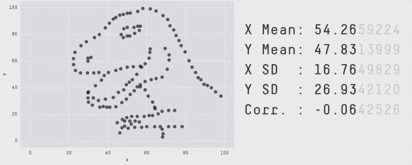
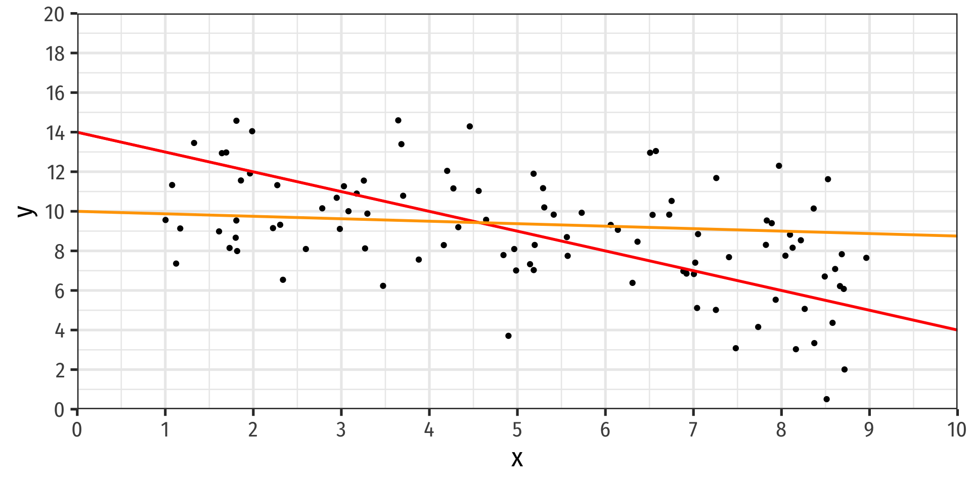
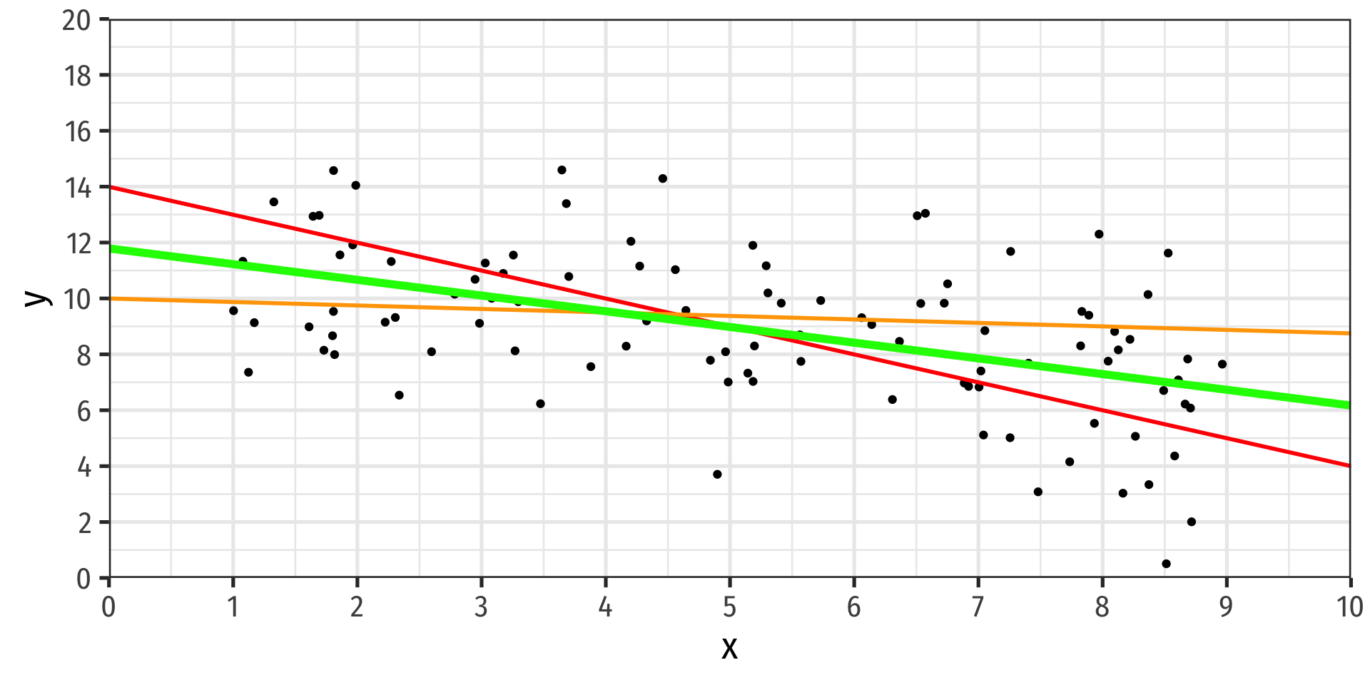
Guess the Correlation!

Correlation and Covariance in R
Correlation and Endogeneity
Your Occasional Reminder: Correlation does not imply causation!
- I’ll show you the difference in a few weeks (when we can actually talk about causation)
If X and Y are strongly correlated, X can still be endogenous!
See today’s appendix page for more on Covariance and Correlation

Always Plot Your Data!
Linear Regression
Fitting a Line to Data
- If an association appears linear, we can estimate the equation of a line that would “fit” the data
Y=a+bX
- A linear equation describing a line has two parameters:
- a: vertical intercept
- b: slope
Fitting a Line to Data
- If an association appears linear, we can estimate the equation of a line that would “fit” the data
Y=a+bX
- A linear equation describing a line has two parameters:
- a: vertical intercept
- b: slope
- How do we choose the equation that best fits the data?
Fitting a Line to Data
- If an association appears linear, we can estimate the equation of a line that would “fit” the data
Y=a+bX
A linear equation describing a line has two parameters:
- a: vertical intercept
- b: slope
How do we choose the equation that best fits the data?
This process is called linear regression
Population Linear Regression Model
Linear regression lets us estimate the slope of the population regression line between X and Y using sample data
We can make statistical inferences about what the true population slope coefficient is
- eventually & hopefully: a causal inference
slope=ΔYΔX: for a 1-unit change in X, how many units will this cause Y to change?
Class Size Example
Example
What is the relationship between class size and educational performance?

Class Size Example: Data Import
Data are student-teacher-ratio and average test scores on Stanford 9 Achievement Test for 5th grade students for 420 K-6 and K-8 school districts in California in 1999, (Stock and Watson, 2015: p. 141)
Class Size Example: Data
Rows: 420
Columns: 21
$ observat <dbl> 1, 2, 3, 4, 5, 6, 7, 8, 9, 10, 11, 12, 13, 14, 15, 16, 17, 18…
$ dist_cod <dbl> 75119, 61499, 61549, 61457, 61523, 62042, 68536, 63834, 62331…
$ county   <chr> "Alameda", "Butte", "Butte", "Butte", "Butte", "Fresno", "San…
$ district <chr> "Sunol Glen Unified", "Manzanita Elementary", "Thermalito Uni…
$ gr_span  <chr> "KK-08", "KK-08", "KK-08", "KK-08", "KK-08", "KK-08", "KK-08"…
$ enrl_tot <dbl> 195, 240, 1550, 243, 1335, 137, 195, 888, 379, 2247, 446, 987…
$ teachers <dbl> 10.90, 11.15, 82.90, 14.00, 71.50, 6.40, 10.00, 42.50, 19.00,…
$ calw_pct <dbl> 0.5102, 15.4167, 55.0323, 36.4754, 33.1086, 12.3188, 12.9032,…
$ meal_pct <dbl> 2.0408, 47.9167, 76.3226, 77.0492, 78.4270, 86.9565, 94.6237,…
$ computer <dbl> 67, 101, 169, 85, 171, 25, 28, 66, 35, 0, 86, 56, 25, 0, 31, …
$ testscr  <dbl> 690.80, 661.20, 643.60, 647.70, 640.85, 605.55, 606.75, 609.0…
$ comp_stu <dbl> 0.34358975, 0.42083332, 0.10903226, 0.34979424, 0.12808989, 0…
$ expn_stu <dbl> 6384.911, 5099.381, 5501.955, 7101.831, 5235.988, 5580.147, 5…
$ str      <dbl> 17.88991, 21.52466, 18.69723, 17.35714, 18.67133, 21.40625, 1…
$ avginc   <dbl> 22.690001, 9.824000, 8.978000, 8.978000, 9.080333, 10.415000,…
$ el_pct   <dbl> 0.000000, 4.583333, 30.000002, 0.000000, 13.857677, 12.408759…
$ read_scr <dbl> 691.6, 660.5, 636.3, 651.9, 641.8, 605.7, 604.5, 605.5, 608.9…
$ math_scr <dbl> 690.0, 661.9, 650.9, 643.5, 639.9, 605.4, 609.0, 612.5, 616.1…
$ aowijef  <dbl> 35.77982, 43.04933, 37.39445, 34.71429, 37.34266, 42.81250, 3…
$ es_pct   <dbl> 1.000000, 3.583333, 29.000002, 1.000000, 12.857677, 11.408759…
$ es_frac  <dbl> 0.01000000, 0.03583334, 0.29000002, 0.01000000, 0.12857677, 0…
Class Size Example: Data
| ABCDEFGHIJ0123456789 |
observat <dbl> | dist_cod <dbl> | county <chr> | district <chr> | gr_span <chr> | |
|---|---|---|---|---|---|
| 1 | 75119 | Alameda | Sunol Glen Unified | KK-08 | |
| 2 | 61499 | Butte | Manzanita Elementary | KK-08 | |
| 3 | 61549 | Butte | Thermalito Union Elementary | KK-08 | |
| 4 | 61457 | Butte | Golden Feather Union Elementary | KK-08 | |
| 5 | 61523 | Butte | Palermo Union Elementary | KK-08 | |
| 6 | 62042 | Fresno | Burrel Union Elementary | KK-08 | |
| 7 | 68536 | San Joaquin | Holt Union Elementary | KK-08 | |
| 8 | 63834 | Kern | Vineland Elementary | KK-08 | |
| 9 | 62331 | Fresno | Orange Center Elementary | KK-08 | |
| 10 | 67306 | Sacramento | Del Paso Heights Elementary | KK-06 |
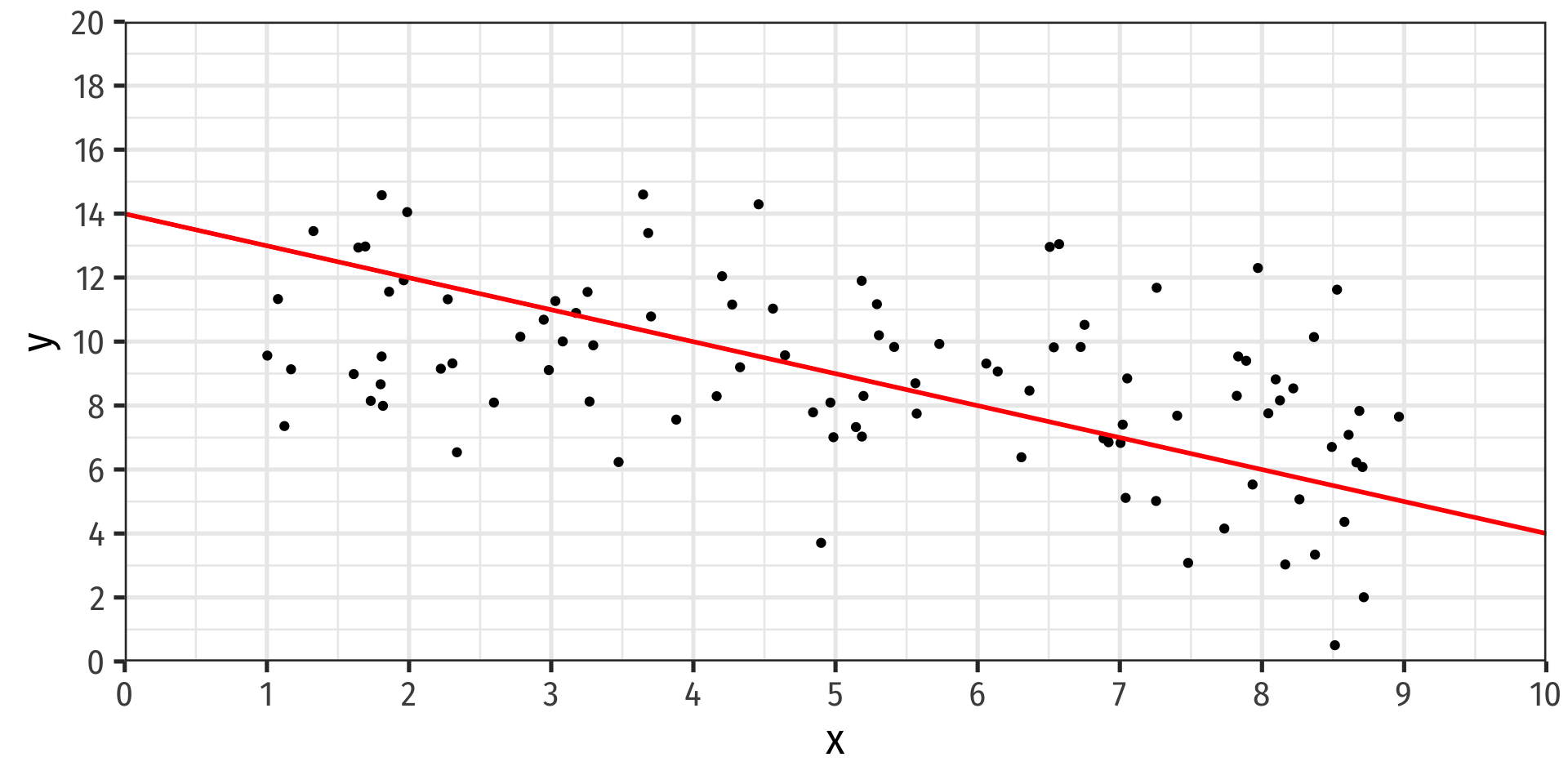
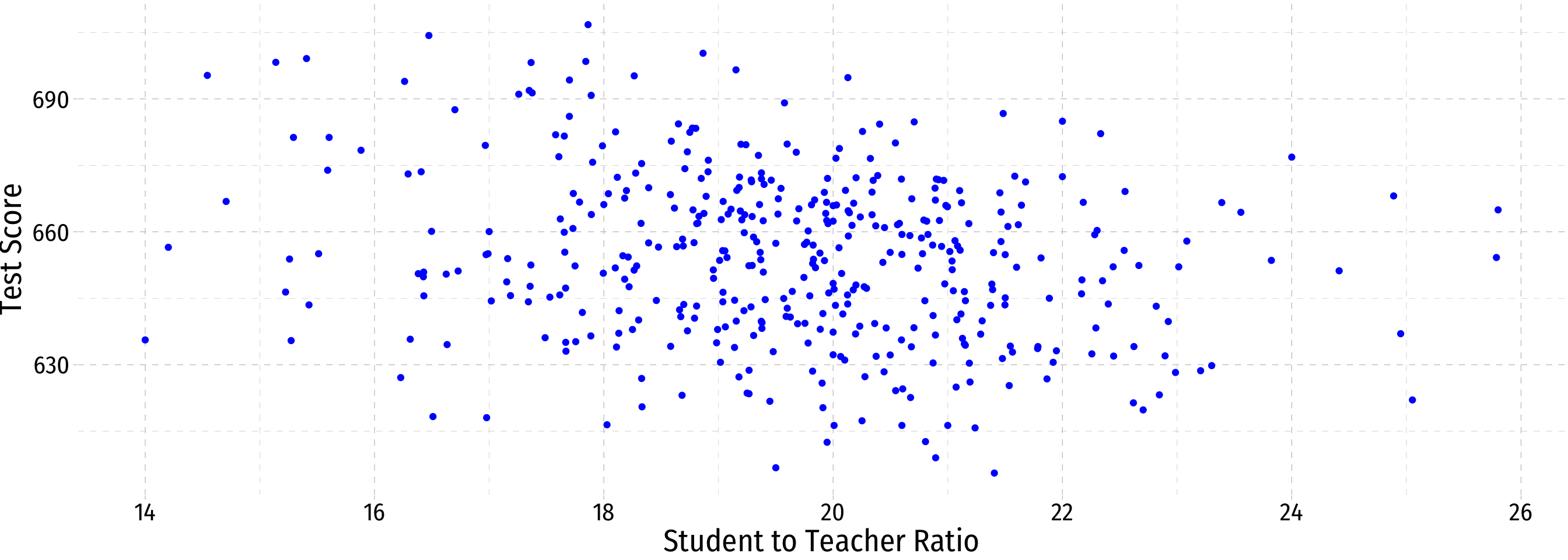
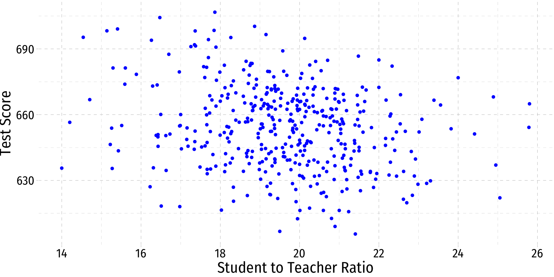
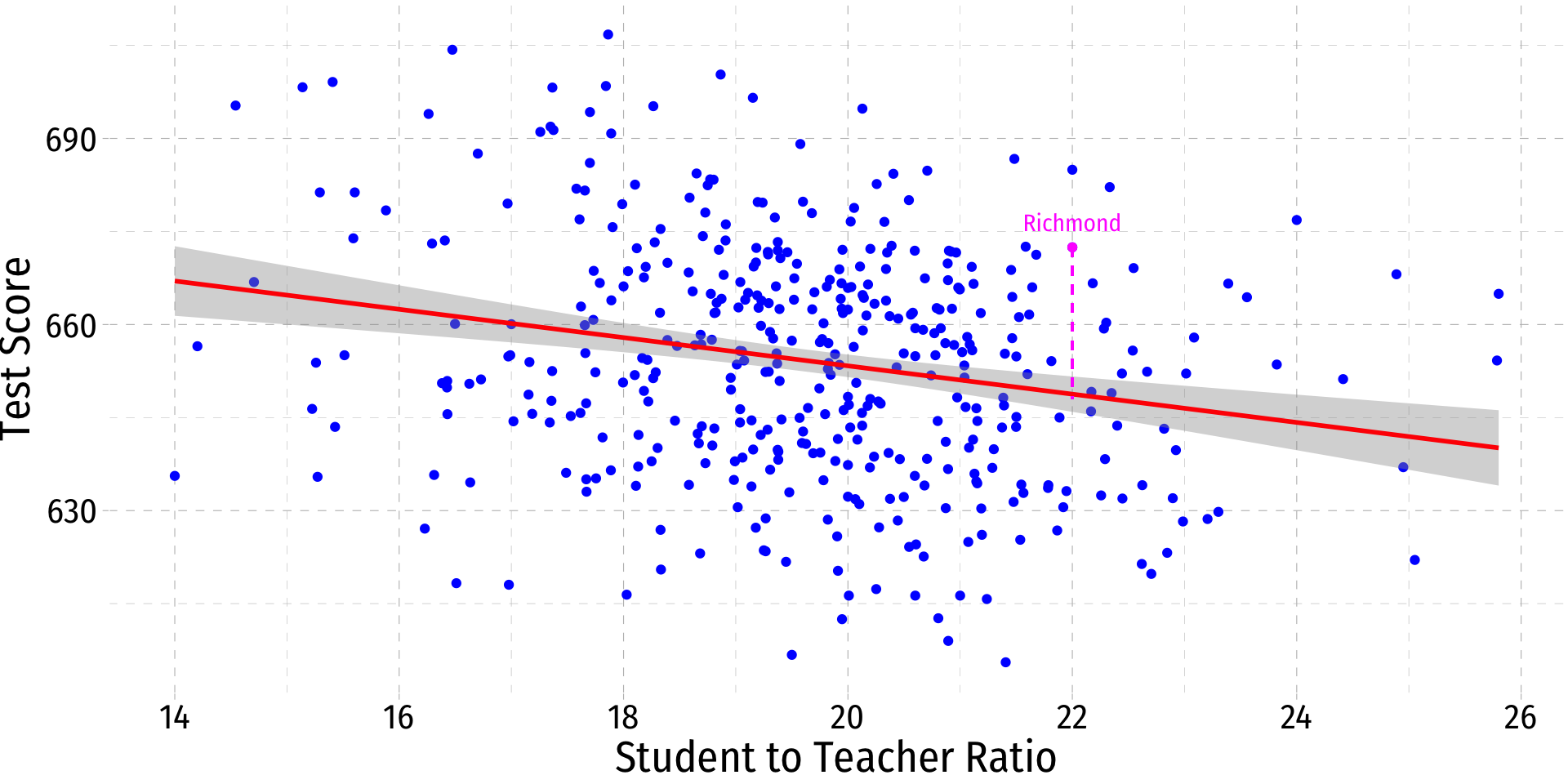
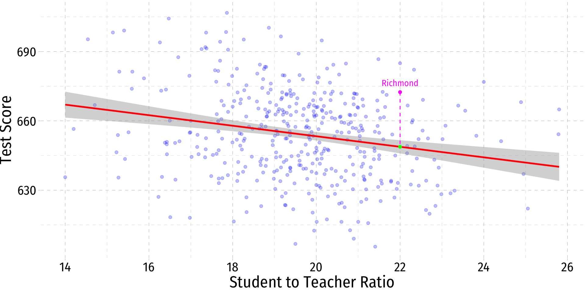
Class Size Example: Scatterplot
Class Size Example: Slope I
- If we change (Δ) the class size by an amount, what would we expect the change in test scores to be?
β=change in test scorechange in class size=Δtest scoreΔclass size
- If we knew β, we could say that changing class size by 1 student will change test scores by β
Class Size Example: Slope II
- Rearranging:
Δtest score=β×Δclass size
Class Size Example: Slope III
- Rearranging:
Δtest score=β×Δclass size
- Suppose β=−0.6. If we shrank class size by 2 students, our model predicts:
Δtest score=−2×βΔtest score=−2×−0.6Δtest score=1.2
Test scores would improve by 1.2 points, on average.
Class Size Example: Slope and Average Effect
test score=β0+β1×class size
The line relating class size and test scores has the above equation
β0 is the vertical-intercept, test score where class size is 0
β1 is the slope of the regression line
This relationship only holds on average for all districts in the population, individual districts are also affected by other factors
Class Size Example: Marginal Effect
- To get an equation that holds for each district, we need to include other factors
test score=β0+β1class size+other factors
For now, we will ignore these until Unit III
Thus, β0+β1class size gives the average effect of class sizes on scores
Later, we will want to estimate the marginal effect (causal effect) of each factor on an individual district’s test score, holding all other factors constant
Econometric Models: Overview I
Y=β0+β1X+u
- Y is the dependent variable of interest
- AKA “response variable,” “regressand,” “Left-hand side (LHS) variable”
- X1 is an independent variable
- AKA “explanatory variable”, “regressor,” “Right-hand side (RHS) variable”, “covariate”
- Our data consists of a spreadsheet of observed values of (X1i,X2i,Yi)
Econometric Models: Overview II
Y=β0+β1X+u
- To model, we “regress Y on X1”
- β0 and β1 are parameters that describe the population relationships between the variables
- unknown! to be estimated
- u is a random error term
- ’U’nobservable, we can’t measure it, and must model with assumptions about it
The Population Regression Model
How do we draw a line through the scatterplot? We do not know the “true” β0 or β1
We do have data from a sample of class sizes and test scores
So the real question is, how can we estimate β0 and β1?

Deriving OLS Estimators
Actual, Predicted, and Residual Values
- With a simple linear regression model, for each associated X value, we have
- The observed (or actual) values of Yi

Actual, Predicted, and Residual Values
- With a simple linear regression model, for each associated X value, we have
- The observed (or actual) values of Yi
- Predicted (or fitted) values, ˆYi
Actual, Predicted, and Residual Values
- With a simple linear regression model, for each associated X value, we have
- The observed (or actual) values of Yi
- Predicted (or fitted) values, ˆYi
- The residual (or error), ˆui=Yi−ˆYi … the difference between predicted and observed values
Yi=ˆYi+ˆuiObservedi=Modeli+Errori
Deriving OLS Estimators
- Take the residuals ˆui and square them (why)?
Deriving OLS Estimators
Take the residuals ˆui and square them (why)?
The regression line minimizes the sum of the squared residuals (SSR)
SSR=n∑i=1ˆui2

O-rdinary L-east S-quares Estimators
- The Ordinary Least Squares (OLS) estimators of the unknown population parameters β0 and β1, solve the calculus problem:
minβ0,β1n∑i=1[Yi−(β0+β1Xi⏟^Yi)⏟^ui]2
- Intuitively, OLS estimators minimize the sum of the squared residuals (distance between the actual values Yi and the predicted values ^Yi) along the estimated regression line
The OLS Regression Line
- The OLS regression line or sample regression line is the linear function constructed using the OLS estimators:
^Yi=^β0+^β1Xi
- ^β0 and ^β1 (“beta 0 hat” & “beta 1 hat”) are the OLS estimators of population parameters β0 and β1 using sample data
- The predicted value of Y given X, based on the regression, is E(Yi|Xi)=^Yi
- The residual or prediction error for the ith observation is the difference between observed Yi and its predicted value, ^ui=Yi−^Yi
The OLS Regression Estimators
- The solution to the SSE minimization problem yields:1
ˆβ0=ˉY−ˆβ1ˉX
ˆβ1=n∑i=1(Xi−ˉX)(Yi−ˉY)n∑i=1(Xi−ˉX)2=sXYs2X=cov(X,Y)var(X)
(Some) Properties of OLS
- The regression line goes through the “center of mass” point (ˉX,ˉY)
- Again, ˆβ0=ˉY−ˆβ1ˉX
- The slope, ˆβ1 has the same sign as the correlation coefficient rX,Y, and is related
ˆβ1=rsYsX
- The residuals sum and average to zero
n∑i=1ˆui=0E[ˆu]=0
- The residuals and X are uncorrelated
Our Class Size Example in R
Class Size Scatterplot (Again)
- There is some true (unknown) population relationship:
test scorei=β0+β1stri
- β1=Δtest scoreΔstr=??
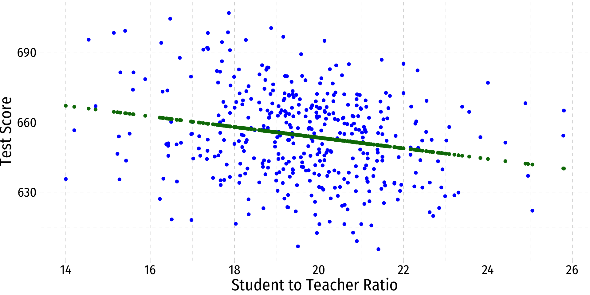
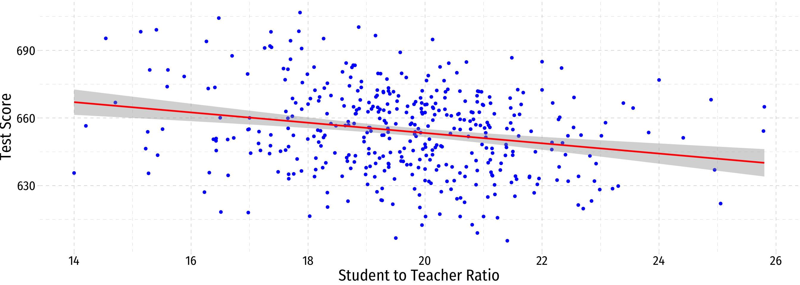
Class Size Scatterplot with Regression Line
Linear Regression in R I
Format for regression is lm(y ~ x, data = df)
yis dependent variable (listed first!)~means “is modeled by” or “is explained by”xis the independent variabledfis name of dataframe where data is stored
This is base R (there’s no good tidyverse way to do this yet…ish1)
Linear Regression in R II
Linear Regression in R II
Call:
lm(formula = testscr ~ str, data = ca_school)

Residuals:
    Min      1Q  Median      3Q     Max
-47.727 -14.251   0.483  12.822  48.540

Coefficients:
            Estimate Std. Error t value Pr(>|t|)
(Intercept) 698.9330     9.4675  73.825  < 2e-16 ***
str          -2.2798     0.4798  -4.751 2.78e-06 ***
---
Signif. codes:  0 '***' 0.001 '**' 0.01 '*' 0.05 '.' 0.1 ' ' 1

Residual standard error: 18.58 on 418 degrees of freedom
Multiple R-squared:  0.05124,   Adjusted R-squared:  0.04897
F-statistic: 22.58 on 1 and 418 DF,  p-value: 2.783e-06
Looking at the
summary, there’s a lot of information here!These objects are cumbersome, come from a much older, pre-
tidyverseera ofbase RLuckily, we now have some more
tidyways of working with regression output!
Tidy Regression with broom

The
broompackage allows us to work with regression objects as tidiertibblesSeveral useful commands:
| Command | Does |
|---|---|
tidy() |
Create tibble of regression coefficients & stats |
glance() |
Create tibble of regression fit statistics |
augment() |
Create tibble of data with regression-based variables |
Tidy Regression with broom: tidy()
- The
tidy()function creates a tidytibbleof regression output
# A tibble: 2 × 5
  term        estimate std.error statistic   p.value
  <chr>          <dbl>     <dbl>     <dbl>     <dbl>
1 (Intercept)   699.       9.47      73.8  6.57e-242
2 str            -2.28     0.480     -4.75 2.78e-  6
Tidy Regression with broom: tidy()
- The
tidy()function creates a tidytibbleof regression output…with confidence intervals
# A tibble: 2 × 7
  term        estimate std.error statistic   p.value conf.low conf.high
  <chr>          <dbl>     <dbl>     <dbl>     <dbl>    <dbl>     <dbl>
1 (Intercept)   699.       9.47      73.8  6.57e-242   680.      718.
2 str            -2.28     0.480     -4.75 2.78e-  6    -3.22     -1.34
Tidy Regression with broom: glance()
glance()shows us a lot of overall regression statistics and diagnostics- We’ll interpret these in next class and beyond
# A tibble: 1 × 12
r.squ…¹ adj.r…² sigma stati…³ p.value df logLik AIC BIC devia…⁴ df.re…⁵
<dbl> <dbl> <dbl> <dbl> <dbl> <dbl> <dbl> <dbl> <dbl> <dbl> <int>
1 0.0512 0.0490 18.6 22.6 2.78e-6 1 -1822. 3650. 3663. 144315. 418
# … with 1 more variable: nobs <int>, and abbreviated variable names
# ¹r.squared, ²adj.r.squared, ³statistic, ⁴deviance, ⁵df.residualTidy Regression with broom: augment()
augment()creates a new tibble with the data (X,Y) and regression-based variables, including:.fittedare fitted (predicted) values from model, i.e. ˆYi.residare residuals (errors) from model, i.e. ˆui
# A tibble: 420 × 8
   testscr   str .fitted .resid    .hat .sigma  .cooksd .std.resid
     <dbl> <dbl>   <dbl>  <dbl>   <dbl>  <dbl>    <dbl>      <dbl>
 1    691.  17.9    658.   32.7 0.00442   18.5 0.00689       1.76
 2    661.  21.5    650.   11.3 0.00475   18.6 0.000893      0.612
 3    644.  18.7    656.  -12.7 0.00297   18.6 0.000700     -0.685
 4    648.  17.4    659.  -11.7 0.00586   18.6 0.00117      -0.629
 5    641.  18.7    656.  -15.5 0.00301   18.6 0.00105      -0.836
 6    606.  21.4    650.  -44.6 0.00446   18.5 0.0130       -2.40
 7    607.  19.5    654.  -47.7 0.00239   18.5 0.00794      -2.57
 8    609   20.9    651.  -42.3 0.00343   18.5 0.00895      -2.28
 9    612.  19.9    653.  -41.0 0.00244   18.5 0.00597      -2.21
10    613.  20.8    652.  -38.9 0.00329   18.5 0.00723      -2.09
# … with 410 more rows
Class Size Regression Result
- Using OLS, we find:
^test scorei=689.93−2.28stri
- ^β0=689.93: test score for str=0
- ^β1=−2.28: for every 1 unit change in str, ^test_score changes by -2.28 points
test scorei=689.93−2.28stri+ˆui
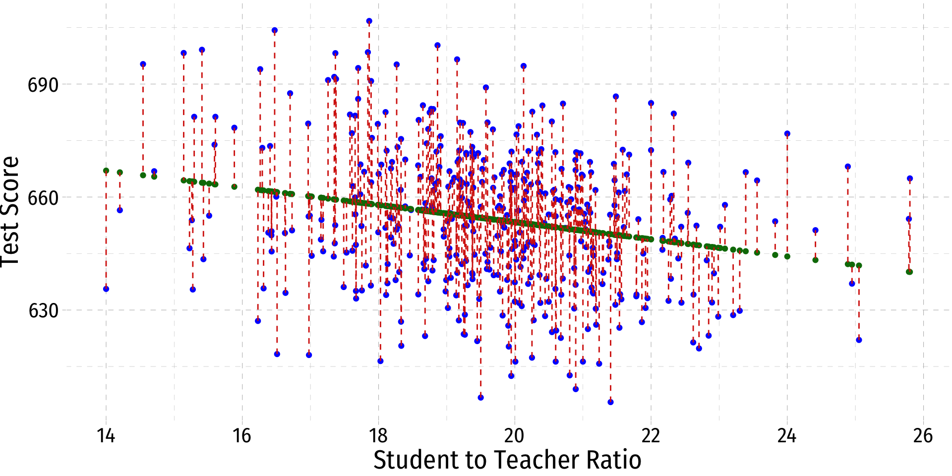
Class Size Regression Residuals
.resid = testscr - .fitted
ˆui=test scorei−^test scorei
ˆui=test scorei−(689.93−2.28stri)
Class Size Regression: Fitted and Residual Values
# A tibble: 420 × 4
   testscr   str .fitted .resid
     <dbl> <dbl>   <dbl>  <dbl>
 1    691.  17.9    658.   32.7
 2    661.  21.5    650.   11.3
 3    644.  18.7    656.  -12.7
 4    648.  17.4    659.  -11.7
 5    641.  18.7    656.  -15.5
 6    606.  21.4    650.  -44.6
 7    607.  19.5    654.  -47.7
 8    609   20.9    651.  -42.3
 9    612.  19.9    653.  -41.0
10    613.  20.8    652.  -38.9
# … with 410 more rows
testscr = .fitted + .resid
Class Size Regression: An Example Data Point I
- One district in our sample is Richmond Elementary
| ABCDEFGHIJ0123456789 |
observat <dbl> | district <chr> | testscr <dbl> | str <dbl> | dist_cod <dbl> | |
|---|---|---|---|---|---|
| 355 | Richmond Elementary | 672.45 | 22 | 64170 |
1 row | 1-5 of 21 columns
Class Size Regression: An Example Data Point II
.fittedvalue:
^Test ScoreRichmond=698−2.28(22)≈648
.residvalue:
ˆuRichmond=672−648≈24
Class Size Regression: An Example Data Point III
Making Predictions
- We can use the regression model to make a prediction for a particular xi
Example
Suppose we have a school district with a student/teacher ratio of 18. What is the predicted average district test score?
^test scorei=^β0+^β1stri=698.93−2.28(18)=657.89
Making Predictions In R
- We can do this in
Rwith thepredict()1 function, which requires (at least) two inputs:- An
lmobject (saved regression) newdatawith X value(s) to predict ˆY for, as adata.frame(ortibble)
- An
# A tibble: 1 × 1
    str
  <dbl>
1 18Making Predictions In R, Manually I
- Of course we could do it ourselves…
Making Predictions In R, Manually II
- Of course we could do it ourselves…
Making Predictions In R, Manually II
- Of course we could do it ourselves…
[1] -2.279808

2.3 — Simple Linear Regression ECON 480 • Econometrics • Fall 2022 Dr. Ryan Safner Associate Professor of Economics safner@hood.edu ryansafner/metricsF22 metricsF22.classes.ryansafner.com