2.4 — Goodness of Fit and Bias

ECON 480 • Econometrics • Fall 2022

Dr. Ryan Safner
Associate Professor of Economics

safner@hood.edu
ryansafner/metricsF22
metricsF22.classes.ryansafner.com

Contents

Goodness of Fit

The Sampling Distributions of the OLS Estimators

Bias and Exogeneity

Actual, Predicted, and Residual Values

• With a simple linear regression model, for each associated \(X\) value, we have

1. The observed (or actual) values of \(\color{#0047AB}{Y_i}\)
2. Predicted (or fitted) values, \(\color{#047806}{\hat{Y}_i}\)
3. The residual (or error), \(\color{#D7250E}{\hat{u}_i}=\color{#0047AB}{Y_i}-\color{#047806}{\hat{Y}_i}\) … the difference between predicted and observed values

\[\begin{align*} \color{#0047AB}{Y_i} &= \color{#047806}{\hat{Y}_i} + \color{#D7250E}{\hat{u}_i} \\ \color{#0047AB}{\text{Observed}_i} &= \color{#047806}{\text{Model}_i} + \color{#D7250E}{\text{Error}_i} \\ \end{align*}\]

“All models are wrong. But some are useful. — George Box”

Goodness of Fit

Goodness of Fit

• How well does a line fit data? How tightly clustered around the line are the data points?

• Quantify how much variation in \(\color{#0047AB}{Y_i}\) is “explained” by the model, \(\color{#047806}{\hat{Y}_i}\)

\[\underbrace{\color{#0047AB}{Y_i}}_{\color{#0047AB}{Observed}}=\underbrace{\color{#047806}{\hat{Y}_i}}_{\color{#047806}{Model}}+\underbrace{\color{#D7250E}{\hat{u}_i}}_{\color{#D7250E}{Error}}\]

• Recall OLS estimators chosen to minimize Sum of Squared Residuals (SSR): \(\left(\displaystyle \sum^n_{i=1}\hat{u_i}^2\right)\)

\(R^2\)

• Primary measure¹ is R-squared, the fraction of variation in \(\color{#0047AB}{Y_i}\) explained by variation in predicted values \(\color{#047806}{\hat{Y}_i}\)

\[R^2 = \frac{var(\color{#047806}{\hat{Y}_i})}{var(\color{#0047AB}{Y_i})}\]

1. Sometimes called the “coefficient of determination”

\(R^2\) Formula I

\[R^2 = \frac{\color{#047806}{SSM}}{\color{#0047AB}{SST}}\]

• Model Sum of Squares (SSM):¹ sum of squared deviations of predicted values from their mean²

\[\color{#047806}{SSM} = \sum^n_{i=1}(\hat{Y_i}-\bar{Y})^2\]

• Total Sum of Squares (TSS): sum of squared deviations of observed values from their mean

\[\color{#0047AB}{SST} = \sum^n_{i=1}(Y_i-\bar{Y})^2\]

1. Sometimes called Explained Sum of Squares (ESS) or Regression Sum of Squares (RSS) in other textbooks.

2. It can be shown that \(\color{#047806}{\bar{\hat{Y_i}}}=\color{#0047AB}{\bar{Y_i}}\)

\(R^2\) Formula II

• Equivalently, \(R^2\) is the complement of the fraction of unexplained variation in \(Y_i\)

\[R^2=1-\left(\frac{\color{#D7250E}{SSR}}{\color{#0047AB}{SST}}\right)\]

• Equivalently, the square of the correlation coefficient between \(X\) and \(Y\)¹:

\[R^2=(r_{X,Y})^2\]

1. The correlation coefficient between \(X\) and \(Y\) is the same as the correlation coefficient between \(Y\) and \(\hat{Y}\): \(r_{X,Y}=r_{Y,\hat{Y}}\), so squaring either would also result in \(R^2\).

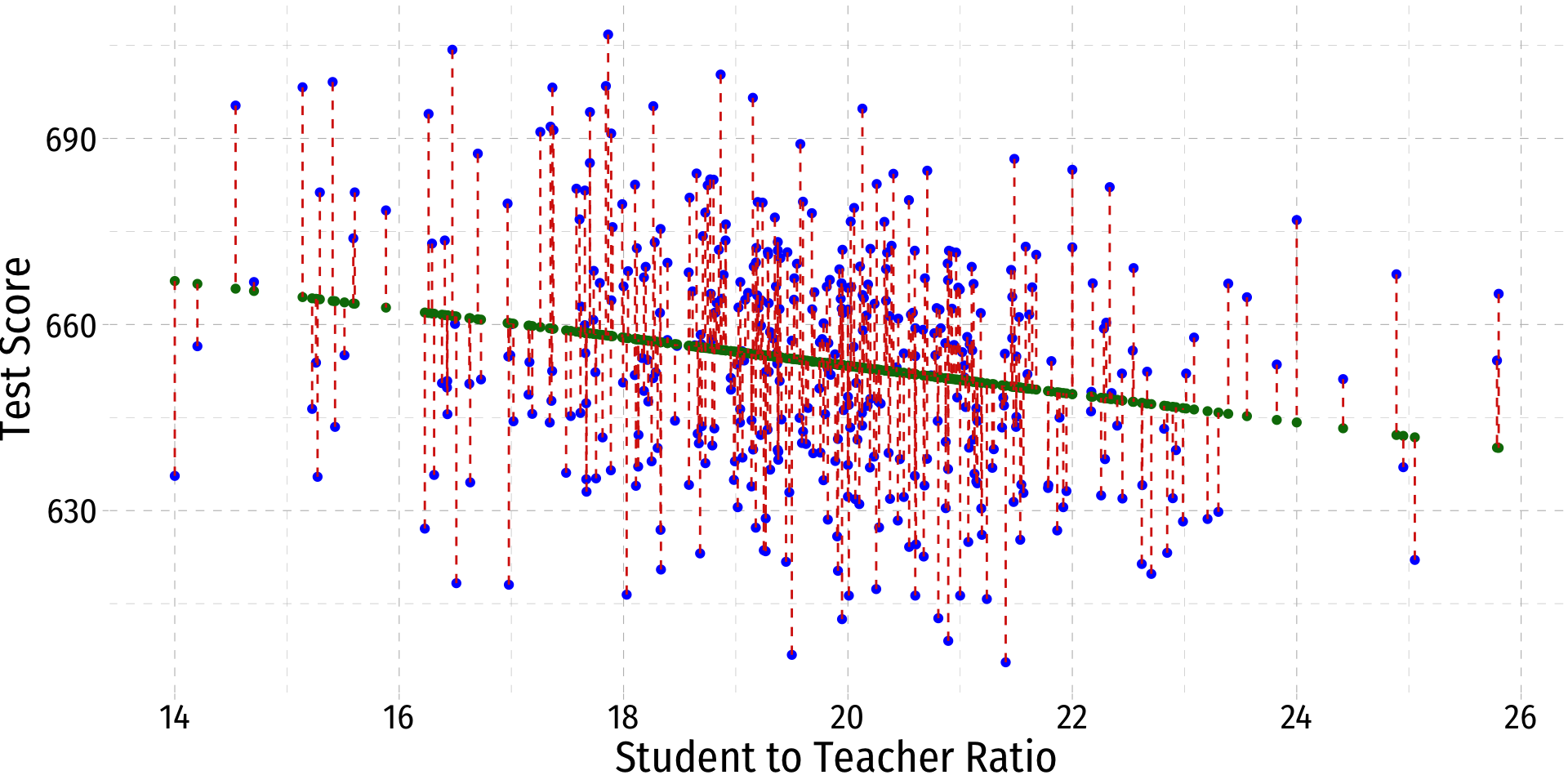
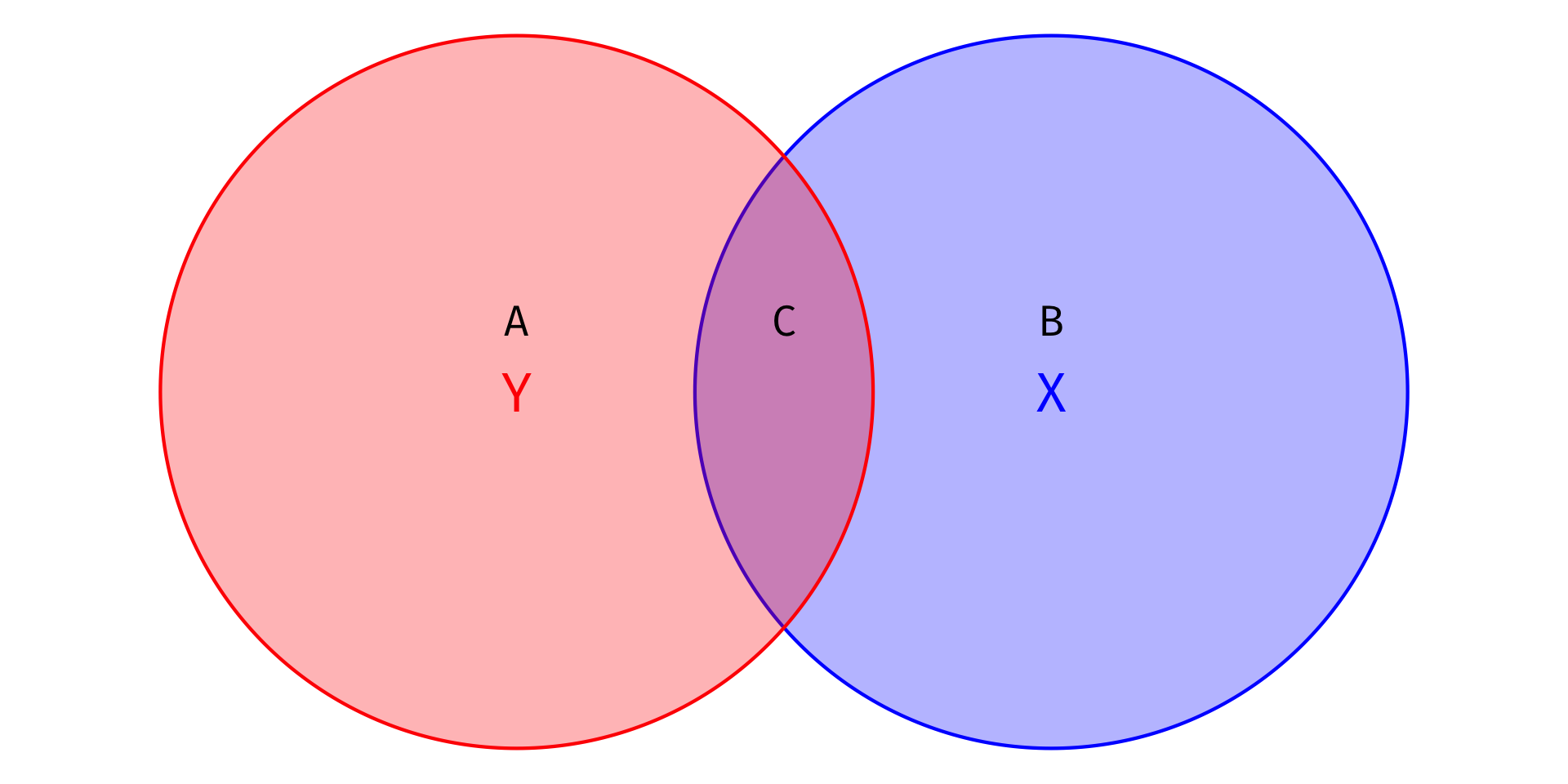
Visualizing \(R^2\) I

• Total Variation in Y: Areas A + C

\[SST = \sum^n_{i=1}(Y_i-\bar{Y})^2\]

• Variation in Y explained by X: Area C

\[\color{#047806}{SSM} = \sum^n_{i=1}(\hat{Y_i}-\bar{Y})^2\]

• Unexplained variation in Y: Area A

\[\color{#D7250E}{SSR} = \sum^n_{i=1}(\hat{u_i})^2\]

\[R^2 = \frac{SSM}{SST} = \frac{\color{purple}{C}}{\color{red}{A}+\color{purple}{C}}\]

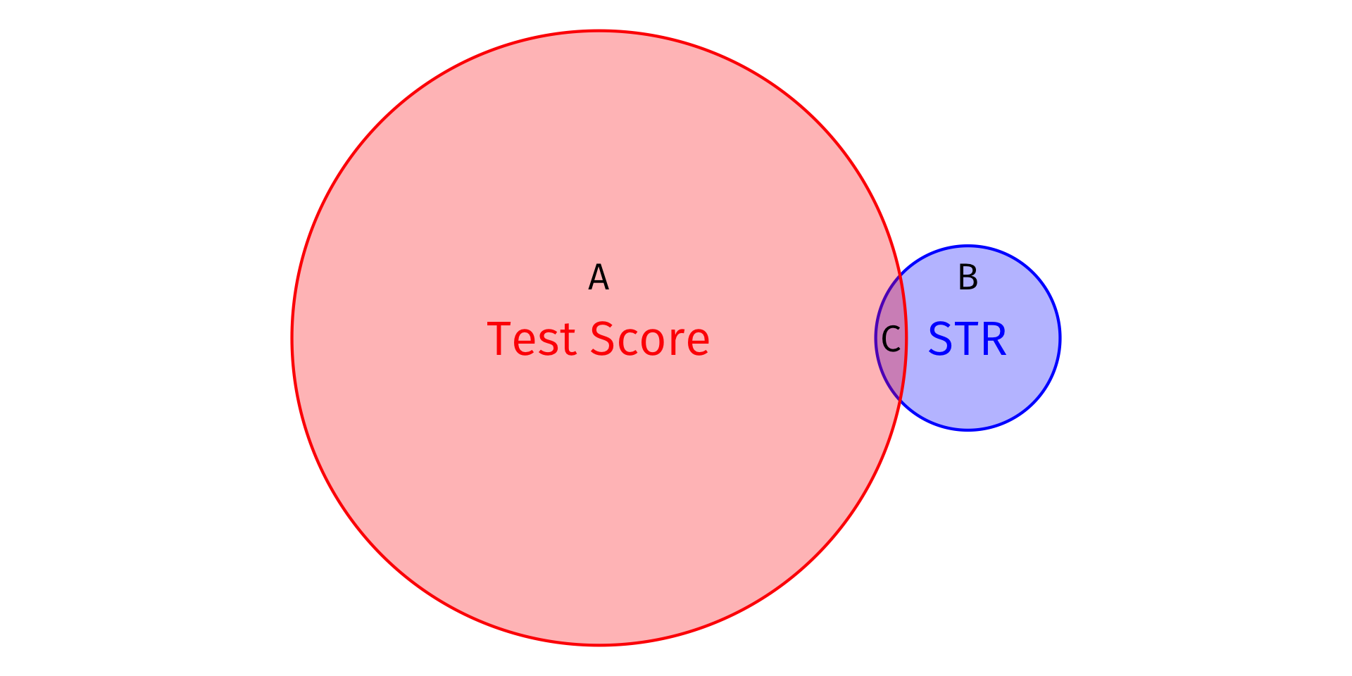
Visualizing \(R^2\) II

# make a function to calc. sum of sq. devs
sum_sq <- function(x){sum((x - mean(x))^2)}

# find total sum of squares
SST <- school_reg %>%
  augment() %>%
  summarize(SST = sum_sq(testscr))

# find explained sum of squares
SSM <- school_reg %>%
  augment() %>%
  summarize(SSM = sum_sq(.fitted))

# look at them and divide to get R^2
tribble(
  ~SSM, ~SST, ~R_sq,
  SSM, SST, SSM/SST
  ) %>%
  knitr::kable()

SSM	SST	R_sq
7794.11	152109.6	0.0512401

\[R^2 = \frac{SSM}{SST} = \frac{\color{purple}{C}}{\color{red}{A}+\color{purple}{C}}=0.05\]

Calculating \(R^2\) in R I

• Recall broom’s augment() command makes a lot of new regression-based values like:
  • .fitted: predicted values \((\hat{Y_i})\)
  • .resid: residuals \((\hat{u_i})\)

library(broom)
school_reg %>%
  augment()

testscr	str	.fitted	.resid	.hat	.sigma	.cooksd	.std.resid
690.80	17.88991	658.1474	32.6526000	0.0044244	18.53408	0.0068925	1.7612148
661.20	21.52466	649.8608	11.3391671	0.0047485	18.59490	0.0008927	0.6117112
643.60	18.69723	656.3069	-12.7068869	0.0029742	18.59279	0.0006996	-0.6848850
647.70	17.35714	659.3620	-11.6619808	0.0058575	18.59441	0.0011673	-0.6294767
640.85	18.67133	656.3659	-15.5159250	0.0030072	18.58766	0.0010548	-0.8363024
605.55	21.40625	650.1308	-44.5807574	0.0044603	18.47411	0.0129531	-2.4046387
606.75	19.50000	654.4767	-47.7266907	0.0023941	18.45548	0.0079356	-2.5716597
609.00	20.89412	651.2984	-42.2983704	0.0034291	18.48716	0.0089463	-2.2803484
612.50	19.94737	653.4568	-40.9567760	0.0024438	18.49453	0.0059658	-2.2069310
612.65	20.80556	651.5003	-38.8502504	0.0032862	18.50537	0.0072306	-2.0943066
615.75	21.23809	650.5142	-34.7641689	0.0040831	18.52485	0.0072052	-1.8747872
616.30	21.00000	651.0570	-34.7569905	0.0036136	18.52492	0.0063680	-1.8739584
616.30	20.60000	651.9689	-35.6689130	0.0029950	18.52080	0.0055515	-1.9225289
616.30	20.00822	653.3181	-37.0180659	0.0024712	18.51448	0.0049285	-1.9947233
616.45	18.02778	657.8331	-41.3830610	0.0041152	18.49207	0.0102908	-2.2317715
617.35	20.25196	652.7624	-35.4123888	0.0026303	18.52202	0.0048022	-1.9083535
618.05	16.97787	660.2267	-42.1766170	0.0071084	18.48740	0.0185757	-2.2779936
618.30	16.50980	661.2938	-42.9937160	0.0089166	18.48263	0.0243010	-2.3242432
619.80	22.70402	647.1721	-27.3721439	0.0086398	18.55446	0.0095387	-1.4795333
620.30	19.91111	653.5394	-33.2394468	0.0024298	18.53171	0.0039069	-1.7910748
620.50	18.33333	657.1365	-36.6364656	0.0035203	18.51621	0.0068913	-1.9751997
621.40	22.61905	647.3659	-25.9658367	0.0082974	18.55936	0.0082379	-1.4032766
621.75	19.44828	654.5946	-32.8446103	0.0024056	18.53340	0.0037763	-1.7697780
622.05	25.05263	641.8178	-19.7677069	0.0219144	18.57747	0.0129635	-1.0757207
622.60	20.67544	651.7969	-29.1969420	0.0030953	18.54804	0.0038451	-1.5737735
623.10	18.68235	656.3408	-33.2407957	0.0029931	18.53166	0.0048183	-1.7916534
623.20	22.84553	646.8495	-23.6495125	0.0092313	18.56681	0.0076172	-1.2786973
623.45	19.26667	655.0086	-31.5586344	0.0024741	18.53877	0.0035862	-1.7005437
623.60	19.25000	655.0466	-31.4466672	0.0024826	18.53923	0.0035731	-1.6945175
624.15	20.54545	652.0933	-27.9432316	0.0029272	18.55269	0.0033295	-1.5060690
624.55	20.60697	651.9530	-27.4029716	0.0030039	18.55462	0.0032865	-1.4770072
624.95	21.07268	650.8913	-25.9412664	0.0037489	18.55965	0.0036811	-1.3987447
625.30	21.53581	649.8354	-24.5354367	0.0047766	18.56421	0.0042044	-1.3236257
625.85	19.90400	653.5556	-27.7056741	0.0024273	18.55357	0.0027114	-1.4928911
626.10	21.19407	650.6145	-24.5145628	0.0039906	18.56430	0.0035010	-1.3219776
626.80	21.86535	649.0841	-22.2840870	0.0056821	18.57102	0.0041331	-1.2027182
626.90	18.32965	657.1449	-30.2448510	0.0035267	18.54397	0.0047052	-1.6306107
627.10	16.22857	661.9349	-34.8349462	0.0101436	18.52405	0.0181933	-1.8843463
627.25	19.17857	655.2095	-27.9594856	0.0025232	18.55265	0.0028710	-1.5066399
627.30	20.27737	652.7044	-25.4044560	0.0026515	18.56148	0.0024914	-1.3690462
628.25	22.98614	646.5290	-18.2789658	0.0098456	18.58147	0.0048593	-0.9886255
628.40	20.44444	652.3235	-23.9235136	0.0028120	18.56620	0.0023440	-1.2893420
628.55	19.82085	653.7452	-25.1951733	0.0024027	18.56217	0.0022195	-1.3575986
628.65	23.20522	646.0295	-17.3794680	0.0108552	18.58354	0.0048531	-0.9404554
628.75	19.26697	655.0080	-26.2579595	0.0024740	18.55863	0.0024826	-1.4149156
629.80	23.30189	645.8091	-16.0090672	0.0113210	18.58652	0.0042987	-0.8665030
630.35	21.18829	650.6277	-20.2777471	0.0039786	18.57661	0.0023882	-1.0934956
630.40	20.87180	651.3493	-20.9492352	0.0033921	18.57483	0.0021706	-1.1293737
630.55	19.01749	655.5767	-25.0267237	0.0026397	18.56271	0.0024071	-1.3486822
630.55	21.91938	648.9610	-18.4109799	0.0058443	18.58124	0.0029028	-0.9937597
631.05	20.10124	653.1060	-22.0559340	0.0025226	18.57177	0.0017862	-1.1885175
631.40	21.47651	649.9706	-18.5706002	0.0046291	18.58089	0.0023335	-1.0017633
631.85	20.06579	653.1868	-21.3368264	0.0025016	18.57379	0.0016576	-1.1497552
631.90	20.37510	652.4816	-20.5816166	0.0027409	18.57584	0.0016907	-1.1091931
631.95	22.44648	647.7593	-15.8092651	0.0076317	18.58699	0.0028050	-0.8540965
632.00	22.89524	646.7362	-14.7361970	0.0094455	18.58910	0.0030274	-0.7968524
632.20	20.49797	652.2015	-20.0014969	0.0028713	18.57736	0.0016732	-1.0779995
632.25	20.00000	653.3368	-21.0867866	0.0024672	18.57448	0.0015966	-1.1362620
632.45	22.25658	648.1922	-15.7422648	0.0069451	18.58714	0.0025275	-0.8501827
632.85	21.56436	649.7703	-16.9203622	0.0048493	18.58468	0.0020303	-0.9128447
632.95	19.47737	654.5283	-21.5782678	0.0023987	18.57313	0.0016253	-1.1627056
633.05	17.67002	658.6487	-25.5987041	0.0049700	18.56074	0.0047638	-1.3811205
633.15	21.94756	648.8967	-15.7466959	0.0059305	18.58715	0.0021551	-0.8499879
633.65	21.78339	649.2710	-15.6209661	0.0054434	18.58741	0.0019447	-0.8429946
633.90	19.14000	655.2974	-21.3973987	0.0025479	18.57362	0.0016981	-1.1530460
634.00	18.11050	657.6445	-23.6444923	0.0039418	18.56702	0.0032168	-1.2750268
634.05	20.68242	651.7810	-17.7309406	0.0031050	18.58290	0.0014225	-0.9557378
634.10	22.62361	647.3555	-13.2554886	0.0083155	18.59181	0.0021516	-0.7163754
634.10	21.78650	649.2639	-15.1639357	0.0054522	18.58833	0.0018356	-0.8183344
634.15	18.58293	656.5674	-22.4174066	0.0031267	18.57071	0.0022899	-1.2083620
634.20	21.54545	649.8134	-15.6134965	0.0048011	18.58744	0.0017114	-0.8423196
634.40	21.15289	650.7084	-16.3083914	0.0039064	18.58602	0.0015165	-0.8794127
634.55	16.63333	661.0121	-26.4621537	0.0084110	18.55766	0.0086750	-1.4301811
634.70	21.14438	650.7278	-16.0278017	0.0038893	18.58660	0.0014583	-0.8642748
634.90	19.78182	653.8342	-18.9341744	0.0023943	18.58006	0.0012491	-1.0202312
634.95	18.98373	655.6537	-20.7037398	0.0026685	18.57551	0.0016654	-1.1157341
635.05	17.66767	658.6541	-23.6040700	0.0049762	18.56711	0.0040554	-1.2735085
635.20	17.75499	658.4550	-23.2550243	0.0047515	18.56818	0.0037570	-1.2545348
635.45	15.27273	664.1141	-28.6640505	0.0151024	18.54939	0.0185256	-1.5544390
635.60	14.00000	667.0156	-31.4156607	0.0235965	18.53797	0.0353765	-1.7110520
635.60	20.59613	651.9777	-16.3777393	0.0029900	18.58589	0.0011685	-0.8827463
635.75	16.31169	661.7454	-25.9954321	0.0097700	18.55920	0.0097510	-1.4059202
635.95	21.12796	650.7652	-14.8152370	0.0038565	18.58903	0.0012354	-0.7988759
636.10	17.48801	659.0636	-22.9636613	0.0054704	18.56903	0.0042238	-1.2392643
636.50	17.88679	658.1545	-21.6544931	0.0044317	18.57285	0.0030364	-1.1680036
636.60	19.30676	654.9172	-18.3172679	0.0024552	18.58154	0.0011989	-0.9870205
636.70	20.89231	651.3025	-14.6025459	0.0034261	18.58944	0.0010653	-0.7872370
636.90	21.28684	650.4030	-13.5030170	0.0041886	18.59143	0.0011153	-0.7282390
636.95	20.19560	652.8909	-15.9408471	0.0025865	18.58681	0.0009568	-0.8590243
637.00	24.95000	642.0517	-5.0517338	0.0211806	18.60155	0.0008170	-0.2748026
637.10	18.13043	657.5990	-20.4990630	0.0039014	18.57602	0.0023929	-1.1053874
637.35	20.00000	653.3368	-15.9868110	0.0024672	18.58671	0.0009177	-0.8614497
637.65	18.72951	656.2333	-18.5832373	0.0029343	18.58090	0.0014762	-1.0015927
637.95	18.25000	657.3265	-19.3764999	0.0036702	18.57893	0.0020103	-1.0447333
637.95	18.99257	655.6335	-17.6835240	0.0026608	18.58301	0.0012114	-0.9529696
638.00	19.88764	653.5929	-15.5929415	0.0024217	18.58752	0.0008569	-0.8402069
638.20	19.37895	654.7527	-16.5526534	0.0024265	18.58552	0.0009675	-0.8919220
638.30	20.46259	652.2822	-13.9821316	0.0028317	18.59059	0.0008063	-0.7535652
638.30	22.29157	648.1124	-9.8123916	0.0070680	18.59698	0.0009996	-0.5299645
638.35	20.70474	651.7301	-13.3801421	0.0031363	18.59165	0.0008183	-0.7212312
638.55	19.06005	655.4797	-16.9296980	0.0026056	18.58470	0.0010872	-0.9123205
638.70	20.23247	652.8068	-14.1067884	0.0026147	18.59037	0.0007575	-0.7602008
639.25	19.69012	654.0432	-14.7932476	0.0023826	18.58909	0.0007587	-0.7971007
639.30	20.36254	652.5103	-13.2102177	0.0027287	18.59195	0.0006934	-0.7119262
639.35	19.75422	653.8971	-14.5471357	0.0023896	18.58956	0.0007359	-0.7838423
639.50	19.37977	654.7508	-15.2508001	0.0024263	18.58820	0.0008212	-0.8217729
639.75	22.92351	646.6717	-6.9217452	0.0095687	18.60012	0.0006768	-0.3743132
639.80	19.37340	654.7653	-14.9653316	0.0024285	18.58876	0.0007915	-0.8063916
639.85	19.15516	655.2629	-15.4128952	0.0025380	18.58788	0.0008776	-0.8305537
639.90	21.30000	650.3730	-10.4730131	0.0042176	18.59613	0.0006756	-0.5648343
640.10	18.30357	657.2043	-17.1043423	0.0035727	18.58430	0.0015246	-0.9221791
640.15	21.07926	650.8763	-10.7262653	0.0037615	18.59579	0.0006315	-0.5783604
640.50	18.79121	656.0926	-15.5926000	0.0028619	18.58751	0.0010135	-0.8403739
640.75	19.62662	654.1880	-13.4380273	0.0023811	18.59156	0.0006257	-0.7240772
640.90	19.59016	654.2711	-13.3711093	0.0023826	18.59168	0.0006199	-0.7204720
641.10	20.87187	651.3491	-10.2491101	0.0033922	18.59644	0.0005196	-0.5525298
641.45	21.11500	650.7948	-9.3448453	0.0038309	18.59758	0.0004882	-0.5038918
641.45	20.08452	653.1441	-11.6941452	0.0025125	18.59439	0.0005001	-0.6301536
641.55	19.91049	653.5409	-11.9908687	0.0024296	18.59394	0.0005084	-0.6461161
641.80	17.81285	658.3231	-16.5230183	0.0046083	18.58555	0.0018389	-0.8913003
642.20	18.13333	657.5924	-15.3924778	0.0038956	18.58790	0.0013471	-0.8300185
642.20	19.22221	655.1100	-12.9099823	0.0024976	18.59246	0.0006059	-0.6956653
642.40	18.66072	656.3901	-13.9900750	0.0030210	18.59058	0.0008615	-0.7540649
642.75	19.60000	654.2487	-11.4987090	0.0023820	18.59469	0.0004583	-0.6195818
643.05	19.28384	654.9695	-11.9195015	0.0024657	18.59405	0.0005098	-0.6422822
643.20	22.81818	646.9119	-3.7119208	0.0091149	18.60234	0.0001852	-0.2006868
643.25	18.80922	656.0515	-12.8015382	0.0028417	18.59264	0.0006783	-0.6899407
643.40	21.37363	650.2052	-6.8051436	0.0043842	18.60024	0.0002966	-0.3670482
643.40	20.02041	653.2903	-9.8902344	0.0024772	18.59691	0.0003527	-0.5329382
643.50	21.49862	649.9202	-6.4202311	0.0046835	18.60056	0.0002822	-0.3463393
643.50	15.42857	663.7588	-20.2587667	0.0142107	18.57638	0.0086918	-1.0981272
643.70	22.40000	647.8652	-4.1652964	0.0074592	18.60211	0.0001902	-0.2250108
643.70	20.12709	653.0471	-9.3470412	0.0025389	18.59759	0.0003229	-0.5036836
644.20	19.03798	655.5300	-11.3300673	0.0026230	18.59494	0.0004902	-0.6105686
644.20	17.34216	659.3962	-15.1961460	0.0059033	18.58826	0.0019977	-0.8202586
644.40	17.01863	660.1337	-15.7337076	0.0069648	18.58716	0.0025321	-0.8497290
644.45	20.80000	651.5129	-7.0629295	0.0032776	18.60001	0.0002383	-0.3807408
644.45	21.15385	650.7062	-6.2562250	0.0039083	18.60070	0.0002233	-0.3373606
644.50	18.45833	656.8515	-12.3514896	0.0033128	18.59337	0.0007368	-0.6658426
644.55	19.14082	655.2955	-10.7455612	0.0025474	18.59577	0.0004282	-0.5790481
644.70	19.40766	654.6872	-9.9872625	0.0024171	18.59679	0.0003508	-0.5381504
644.95	19.56896	654.3195	-9.3694538	0.0023844	18.59756	0.0003046	-0.5048523
645.10	21.50120	649.9143	-4.8143634	0.0046899	18.60173	0.0001589	-0.2597116
645.25	17.52941	658.9693	-13.7192551	0.0053527	18.59103	0.0014748	-0.7403339
645.55	16.43017	661.4753	-15.9253223	0.0092534	18.58673	0.0034625	-0.8610703
645.55	19.79654	653.8006	-8.2505891	0.0023972	18.59883	0.0002375	-0.4445676
645.60	17.18613	659.7519	-14.1518853	0.0063978	18.59024	0.0018796	-0.7640815
645.75	17.61589	658.7721	-13.0220905	0.0051142	18.59224	0.0012689	-0.7026285
645.75	20.12537	653.0510	-7.3009626	0.0025378	18.59979	0.0001969	-0.3934265
646.00	22.16667	648.3972	-2.3972034	0.0066367	18.60286	0.0000560	-0.1294442
646.20	19.96154	653.4245	-7.2244596	0.0024497	18.59986	0.0001861	-0.3892868
646.35	19.03945	655.5267	-9.1766772	0.0026218	18.59779	0.0003214	-0.4945238
646.40	15.22436	664.2243	-17.8243069	0.0153857	18.58242	0.0073020	-0.9667435
646.50	21.14475	650.7270	-4.2269747	0.0038900	18.60208	0.0001014	-0.2279332
646.55	19.64390	654.1486	-7.5986387	0.0023810	18.59950	0.0002000	-0.4094351
646.70	21.04869	650.9460	-4.2459648	0.0037035	18.60207	0.0000974	-0.2289358
646.90	20.17544	652.9368	-6.0367973	0.0025718	18.60088	0.0001364	-0.3253100
646.95	21.39130	650.1649	-3.2149290	0.0044252	18.60256	0.0000668	-0.1734068
647.05	20.00833	653.3178	-6.2678181	0.0024712	18.60070	0.0001413	-0.3377422
647.25	20.29137	652.6725	-5.4225136	0.0026635	18.60133	0.0001140	-0.2922210
647.30	17.66667	658.6563	-11.3563529	0.0049788	18.59488	0.0009392	-0.6127092
647.60	18.22055	657.3936	-9.7936146	0.0037254	18.59703	0.0005213	-0.5280623
647.60	20.27100	652.7190	-5.1189788	0.0026461	18.60154	0.0001010	-0.2758610
648.00	20.19895	652.8832	-4.8832278	0.0025890	18.60169	0.0000899	-0.2631489
648.20	21.38424	650.1810	-1.9809613	0.0044088	18.60298	0.0000253	-0.1068482
648.25	20.97368	651.1170	-2.8669730	0.0035663	18.60270	0.0000428	-0.1545721
648.35	20.00000	653.3368	-4.9868110	0.0024672	18.60163	0.0000893	-0.2687144
648.70	17.15328	659.8268	-11.1267409	0.0065060	18.59520	0.0011818	-0.6007822
648.95	22.34977	647.9798	0.9701931	0.0072760	18.60317	0.0000101	0.0524053
649.15	22.17007	648.3894	0.7605829	0.0066482	18.60320	0.0000056	0.0410702
649.30	18.18182	657.4819	-8.1818441	0.0037997	18.59890	0.0003712	-0.4411736
649.50	18.95714	655.7143	-6.2142988	0.0026923	18.60074	0.0001514	-0.3348954
649.70	19.74533	653.9174	-4.2174323	0.0023883	18.60208	0.0000618	-0.2272475
649.85	16.42623	661.4843	-11.6343227	0.0092702	18.59443	0.0018514	-0.6290645
650.45	16.62540	661.0302	-10.5802839	0.0084429	18.59596	0.0013921	-0.5718342
650.55	16.38177	661.5857	-11.0356758	0.0094622	18.59531	0.0017009	-0.5967536
650.60	20.07416	653.1677	-2.5677456	0.0025064	18.60281	0.0000241	-0.1383658
650.65	17.99544	657.9068	-7.2567670	0.0041854	18.59982	0.0003219	-0.3913683
650.90	19.39130	654.7245	-3.8244723	0.0024223	18.60229	0.0000516	-0.2060772
650.90	16.42857	661.4790	-10.5789340	0.0092602	18.59595	0.0015290	-0.5719970
651.15	16.72949	660.7929	-9.6429060	0.0080316	18.59719	0.0010991	-0.5210635
651.20	24.41345	643.2750	7.9250504	0.0175731	18.59911	0.0016561	0.4303121
651.35	18.26415	657.2942	-5.9442148	0.0036441	18.60095	0.0001878	-0.3204933
651.40	18.95504	655.7191	-4.3190663	0.0026942	18.60203	0.0000732	-0.2327595
651.45	21.03896	650.9682	0.4818585	0.0036853	18.60322	0.0000012	0.0259808
651.80	20.74074	651.6480	0.1520070	0.0031883	18.60323	0.0000001	0.0081939
651.85	18.10000	657.6684	-5.8184459	0.0039633	18.60104	0.0001959	-0.3137625
651.90	19.84615	653.6875	-1.7875032	0.0024092	18.60303	0.0000112	-0.0963169
652.00	21.60000	649.6891	2.3109075	0.0049416	18.60289	0.0000386	0.1246780
652.10	22.44242	647.7685	4.3314405	0.0076165	18.60201	0.0002101	0.2340045
652.10	23.01438	646.4646	5.6353877	0.0099721	18.60117	0.0004679	0.3048118
652.30	17.74892	658.4688	-6.1688330	0.0047668	18.60077	0.0002652	-0.3327915
652.30	18.28664	657.2429	-4.9428697	0.0036031	18.60165	0.0001284	-0.2664984
652.35	19.26544	655.0114	-2.6614627	0.0024747	18.60278	0.0000255	-0.1434135
652.40	22.66667	647.2573	5.1427251	0.0084881	18.60151	0.0003307	0.2779560
652.40	19.29412	654.9461	-2.5460401	0.0024609	18.60281	0.0000232	-0.1371930
652.50	17.36364	659.3472	-6.8471910	0.0058378	18.60019	0.0004010	-0.3695860
652.85	19.82143	653.7439	-0.8939202	0.0024028	18.60318	0.0000028	-0.0481674
653.10	20.43378	652.3479	0.7521214	0.0028007	18.60320	0.0000023	0.0405349
653.40	21.03721	650.9721	2.4278745	0.0036820	18.60285	0.0000317	0.1309058
653.50	19.92462	653.5086	-0.0086306	0.0024348	18.60323	0.0000000	-0.0004651
653.55	19.00986	655.5941	-2.0441346	0.0026461	18.60296	0.0000161	-0.1101581
653.55	23.82222	644.6229	8.9271951	0.0140425	18.59802	0.0016672	0.4838576
653.70	19.36909	654.7752	-1.0751999	0.0024300	18.60316	0.0000041	-0.0579361
653.80	19.82857	653.7276	0.0723767	0.0024046	18.60323	0.0000000	0.0038999
653.85	15.25885	664.1457	-10.2957130	0.0151833	18.59629	0.0024033	-0.5583550
653.95	17.16129	659.8085	-5.8585474	0.0064795	18.60101	0.0003263	-0.3163248
654.10	21.81333	649.2027	4.8972418	0.0055295	18.60168	0.0001942	0.2642940
654.20	19.07471	655.4463	-1.2463129	0.0025944	18.60313	0.0000059	-0.0671619
654.20	25.78512	640.1478	14.0521378	0.0275595	18.59014	0.0083342	0.7669068
654.30	18.21261	657.4117	-3.1116961	0.0037404	18.60261	0.0000528	-0.1677809
654.60	18.16606	657.5178	-2.9178351	0.0038305	18.60268	0.0000476	-0.1573352
654.85	16.97297	660.2378	-5.3878525	0.0071258	18.60135	0.0003039	-0.2910049
654.85	21.50087	649.9151	4.9348930	0.0046891	18.60166	0.0001669	0.2662135
654.90	20.60000	651.9689	2.9311237	0.0029950	18.60268	0.0000375	0.1579855
655.05	16.99029	660.1983	-5.1483570	0.0070644	18.60151	0.0002750	-0.2780608
655.05	20.77954	651.5596	3.4904750	0.0032463	18.60245	0.0000577	0.1881578
655.05	15.51247	663.5675	-8.5174540	0.0137442	18.59849	0.0014845	-0.4615797
655.20	19.88506	653.5988	1.6011176	0.0024209	18.60307	0.0000090	0.0862743
655.30	21.39882	650.1477	5.1523100	0.0044428	18.60151	0.0001723	0.2779077
655.35	20.49751	652.2026	3.1474228	0.0028708	18.60259	0.0000414	0.1696333
655.35	19.36376	654.7873	0.5626794	0.0024320	18.60321	0.0000011	0.0303195
655.40	17.65957	658.6725	-3.2724836	0.0049975	18.60254	0.0000783	-0.1765619
655.55	21.01796	651.0160	4.5339452	0.0036464	18.60190	0.0001094	0.2444563
655.70	19.05565	655.4897	0.2102249	0.0026090	18.60323	0.0000002	0.0113288
655.80	22.53846	647.5496	8.2504072	0.0079816	18.59881	0.0007995	0.4458073
655.85	21.10787	650.8111	5.0389248	0.0038170	18.60159	0.0001414	0.2717065
656.40	20.05135	653.2197	3.1803139	0.0024936	18.60258	0.0000367	0.1713736
656.50	14.20176	666.5557	-10.0556550	0.0221058	18.59657	0.0033851	-0.5472630
656.55	18.47687	656.8092	-0.2591875	0.0032838	18.60323	0.0000003	-0.0139720
656.65	18.63542	656.4478	0.2022480	0.0030545	18.60323	0.0000002	0.0109013
656.70	20.94595	651.1802	5.5198006	0.0035175	18.60126	0.0001563	0.2975913
656.80	21.08548	650.8621	5.9379523	0.0037735	18.60095	0.0001941	0.3201764
656.80	18.69288	656.3168	0.4832807	0.0029797	18.60322	0.0000010	0.0260483
657.00	20.86808	651.3577	5.6422654	0.0033860	18.60117	0.0001572	0.3041737
657.00	19.82558	653.7344	3.2655619	0.0024038	18.60254	0.0000373	0.1759593
657.15	19.75000	653.9067	3.2432858	0.0023890	18.60255	0.0000366	0.1747577
657.40	19.50000	654.4767	2.9233337	0.0023941	18.60268	0.0000298	0.1575181
657.50	18.39080	657.0054	0.4945557	0.0034223	18.60322	0.0000012	0.0266619
657.55	18.78676	656.1027	1.4473171	0.0028669	18.60310	0.0000087	0.0780043
657.65	19.77018	653.8607	3.7892917	0.0023922	18.60231	0.0000500	0.2041784
657.75	19.33333	654.8567	2.8933427	0.0024438	18.60269	0.0000298	0.1559060
657.80	21.46392	649.9993	7.8006508	0.0045983	18.59929	0.0004090	0.4207880
657.90	23.08492	646.3038	11.5962704	0.0102929	18.59447	0.0020464	0.6273309
658.00	21.06299	650.9134	7.0866316	0.0037305	18.59998	0.0002734	0.3821053
658.35	18.68687	656.3305	2.0195013	0.0029873	18.60297	0.0000178	0.1088493
658.60	20.77024	651.5808	7.0191773	0.0032322	18.60005	0.0002321	0.3783736
658.80	19.30556	654.9200	3.8800005	0.0024557	18.60226	0.0000538	0.2090727
659.05	20.13280	653.0340	6.0160275	0.0025426	18.60089	0.0001340	0.3241860
659.15	20.66964	651.8101	7.3398790	0.0030873	18.59975	0.0002424	0.3956326
659.35	22.28155	648.1353	11.2146930	0.0070326	18.59507	0.0012991	0.6056916
659.40	20.60027	651.9683	7.4317411	0.0029953	18.59966	0.0002410	0.4005656
659.40	20.82734	651.4506	7.9494125	0.0033204	18.59915	0.0003059	0.4285376
659.80	19.22492	655.1038	4.6961767	0.0024961	18.60181	0.0000801	0.2530573
659.90	17.65477	658.6835	1.2165628	0.0050102	18.60314	0.0000108	0.0656382
660.05	17.00000	660.1762	-0.1261626	0.0070301	18.60323	0.0000002	-0.0068139
660.10	16.49773	661.3213	-1.2213189	0.0089672	18.60314	0.0000197	-0.0660263
660.20	19.78261	653.8324	6.3675526	0.0023944	18.60061	0.0001413	0.3431032
660.30	22.30216	648.0883	12.2116809	0.0071055	18.59355	0.0015566	0.6595619
660.75	17.73077	658.5102	2.2398043	0.0048128	18.60291	0.0000353	0.1208341
660.95	20.44836	652.3146	8.6353404	0.0028162	18.59841	0.0003059	0.4653970
661.35	20.37169	652.4894	8.8605813	0.0027376	18.59816	0.0003130	0.4775174
661.45	20.16479	652.9611	8.4889091	0.0025643	18.59858	0.0002690	0.4574473
661.60	21.61538	649.6540	11.9459398	0.0049820	18.59399	0.0010400	0.6445202
661.60	20.56143	652.0568	9.5431374	0.0029466	18.59735	0.0003909	0.5143558
661.85	19.95551	653.4382	8.4117628	0.0024472	18.59866	0.0002520	0.4532635
661.85	21.18387	650.6378	11.2121864	0.0039695	18.59510	0.0007285	0.6046244
661.85	18.81042	656.0488	5.8011813	0.0028404	18.60106	0.0001392	0.3126553
661.90	20.57838	652.0182	9.8818390	0.0029676	18.59692	0.0004222	0.5326168
661.90	18.32461	657.1564	4.7436649	0.0035355	18.60178	0.0001160	0.2557495
661.95	18.82063	656.0255	5.9244818	0.0028291	18.60096	0.0001446	0.3192988
662.40	20.81633	651.4757	10.9243049	0.0033030	18.59551	0.0005747	0.5889032
662.40	20.00000	653.3368	9.0632378	0.0024672	18.59793	0.0002949	0.4883728
662.45	19.68182	654.0622	8.3878317	0.0023821	18.59869	0.0002439	0.4519592
662.50	19.39018	654.7271	7.7729334	0.0024227	18.59933	0.0002130	0.4188354
662.55	20.92732	651.2227	11.3273708	0.0034853	18.59493	0.0006522	0.6106874
662.55	19.94437	653.4636	9.0864284	0.0024426	18.59790	0.0002935	0.4896164
662.65	20.79109	651.5332	11.1167801	0.0032639	18.59524	0.0005880	0.5992673
662.70	19.20354	655.1526	7.5474470	0.0025082	18.59955	0.0002080	0.4067027
662.75	19.02439	655.5610	7.1890123	0.0026340	18.59989	0.0001982	0.3874125
662.90	17.62058	658.7614	4.1386136	0.0051016	18.60212	0.0001278	0.2233043
663.35	20.23715	652.7961	10.5538547	0.0026184	18.59603	0.0004246	0.5687378
663.45	19.29374	654.9469	8.5030256	0.0024611	18.59856	0.0002590	0.4581843
663.50	18.82998	656.0042	7.4957941	0.0028190	18.59960	0.0002307	0.4039823
663.85	20.33949	652.5628	11.2871675	0.0027068	18.59500	0.0005021	0.6082824
663.85	19.22900	655.0945	8.7554483	0.0024938	18.59828	0.0002782	0.4717938
663.90	17.89130	658.1442	5.7558152	0.0044211	18.60109	0.0002140	0.3104565
664.00	19.51881	654.4338	9.5661931	0.0023908	18.59732	0.0003184	0.5154548
664.00	19.08451	655.4239	8.5760649	0.0025870	18.59848	0.0002770	0.4621492
664.15	19.93548	653.4839	10.6661536	0.0024390	18.59588	0.0004038	0.5747378
664.15	18.87326	655.9055	8.2444791	0.0027734	18.59884	0.0002745	0.4443222
664.30	20.14178	653.0135	11.2864431	0.0025486	18.59500	0.0004726	0.6081951
664.40	23.55637	645.2289	19.1710835	0.0126069	18.57923	0.0068826	1.0383250
664.45	21.46479	649.9973	14.4526014	0.0046004	18.58970	0.0014045	0.7796128
664.70	19.19101	655.1811	9.5188868	0.0025156	18.59738	0.0003318	0.5129379
664.75	20.13080	653.0386	11.7114129	0.0025413	18.59437	0.0005074	0.6310932
664.95	25.80000	640.1139	24.8360509	0.0276816	18.56230	0.0261561	1.3555326
664.95	18.77774	656.1233	8.8267082	0.0028772	18.59820	0.0003265	0.4757252
665.10	19.10982	655.3662	9.7337392	0.0025687	18.59711	0.0003543	0.5245295
665.20	19.70109	654.0183	11.1817591	0.0023834	18.59515	0.0004336	0.6025041
665.35	18.61594	656.4922	8.8578021	0.0030809	18.59816	0.0003522	0.4774498
665.65	20.99721	651.0633	14.5866888	0.0036085	18.58946	0.0011200	0.7864541
665.90	20.00000	653.3368	12.5632378	0.0024672	18.59303	0.0005667	0.6769704
665.95	20.98325	651.0952	14.8548507	0.0035834	18.58895	0.0011534	0.8009022
666.00	21.64262	649.5919	16.4080810	0.0050542	18.58578	0.0019907	0.8852986
666.05	20.02967	653.2691	12.7809101	0.0024820	18.59268	0.0005901	0.6887048
666.10	19.81140	653.7668	12.3332116	0.0024004	18.59340	0.0005313	0.6645532
666.15	18.00000	657.8964	8.2536213	0.0041755	18.59882	0.0004154	0.4451279
666.15	19.35811	654.8002	11.3498483	0.0024341	18.59491	0.0004563	0.6115767
666.45	20.17912	652.9284	13.5215262	0.0025745	18.59142	0.0006852	0.7286469
666.55	21.11986	650.7837	15.7663364	0.0038405	18.58714	0.0013932	0.8501548
666.60	23.38974	645.6088	20.9911376	0.0117551	18.57447	0.0076807	1.1364108
666.65	22.18182	648.3627	18.2873646	0.0066879	18.58152	0.0032829	0.9875065
666.65	19.94283	653.4671	13.1828949	0.0024419	18.59200	0.0006176	0.7103516
666.70	17.78826	658.3791	8.3208116	0.0046686	18.59875	0.0004725	0.4488627
666.85	14.70588	665.4064	1.4436151	0.0186186	18.60310	0.0000583	0.0784267
666.85	19.04077	655.5237	11.3263232	0.0026207	18.59494	0.0004895	0.6103662
667.15	20.89195	651.3033	15.8467229	0.0034255	18.58699	0.0012543	0.8543115
667.20	19.83851	653.7050	13.4949908	0.0024071	18.59146	0.0006379	0.7271560
667.45	19.52191	654.4267	13.0232758	0.0023903	18.59227	0.0005899	0.7017325
667.45	20.68622	651.7723	15.6776717	0.0031103	18.58734	0.0011140	0.8450642
667.60	18.18182	657.4819	10.1180826	0.0037997	18.59661	0.0005677	0.5455776
668.00	18.89224	655.8623	12.1377385	0.0027542	18.59371	0.0005909	0.6541365
668.10	24.88889	642.1911	25.9089194	0.0207503	18.55900	0.0210363	1.4090755
668.40	18.58064	656.5726	11.8273796	0.0031299	18.59419	0.0006381	0.6375305
668.60	18.04000	657.8052	10.7947668	0.0040890	18.59569	0.0006957	0.5821497
668.65	17.73399	658.5029	10.1471688	0.0048046	18.59656	0.0007234	0.5474222
668.80	21.45455	650.0207	18.7792872	0.0045756	18.58038	0.0023584	1.0129934
668.90	19.92343	653.5114	15.3886630	0.0024344	18.58793	0.0008390	0.8292048
668.95	20.33942	652.5630	16.3870389	0.0027068	18.58587	0.0010584	0.8831220
669.10	22.54608	647.5322	21.5677538	0.0080111	18.57299	0.0054843	1.1654219
669.30	21.10344	650.8211	18.4789011	0.0038083	18.58113	0.0018977	0.9964061
669.30	18.19743	657.4463	11.8537387	0.0037695	18.59414	0.0007729	0.6391564
669.35	20.10768	653.0913	16.2586817	0.0025265	18.58614	0.0009721	0.8761255
669.35	19.15984	655.2522	14.0977757	0.0025350	18.59039	0.0007334	0.7596848
669.80	19.54545	654.3731	15.4269235	0.0023870	18.58785	0.0008266	0.8312467
669.85	20.88889	651.3103	18.5396862	0.0034204	18.58099	0.0017143	0.9994891
669.95	18.39150	657.0039	12.9461594	0.0034211	18.59239	0.0008361	0.6979379
670.00	19.17990	655.2065	14.7935495	0.0025224	18.58909	0.0008035	0.7971728
670.70	19.39771	654.7099	15.9900520	0.0024202	18.58671	0.0009005	0.8616041
671.25	21.67827	649.5106	21.7393524	0.0051503	18.57259	0.0035616	1.1730041
671.30	19.28889	654.9580	16.3420043	0.0024634	18.58597	0.0009574	0.8805876
671.60	20.34927	652.5405	19.0594660	0.0027160	18.57974	0.0014366	1.0271479
671.60	20.96416	651.1387	20.4612911	0.0035495	18.57613	0.0021675	1.1031558
671.65	19.46039	654.5670	17.0830307	0.0024026	18.58437	0.0010203	0.9204897
671.70	19.28572	654.9652	16.7347320	0.0024649	18.58513	0.0010046	0.9017504
671.75	20.91979	651.2398	20.5101676	0.0034724	18.57601	0.0021302	1.1057482
671.90	20.90021	651.2845	20.6155514	0.0034393	18.57573	0.0021315	1.1114112
671.90	20.59575	651.9786	19.9214224	0.0029895	18.57756	0.0017285	1.0737475
671.95	19.37500	654.7617	17.1882844	0.0024279	18.58414	0.0010439	0.9261729
672.05	19.95122	653.4480	18.6019998	0.0024454	18.58086	0.0012315	1.0023582
672.05	18.84973	655.9592	16.0908748	0.0027979	18.58649	0.0010550	0.8672009
672.30	18.11787	657.6277	14.6723064	0.0039268	18.58930	0.0012339	0.7911967
672.35	19.18341	655.1985	17.1515175	0.0025202	18.58422	0.0010791	0.9242345
672.45	22.00000	648.7772	23.6728422	0.0060937	18.56686	0.0050064	1.2779368
672.55	21.58416	649.7252	22.8248386	0.0049004	18.56946	0.0037338	1.2314197
672.70	20.38889	652.4502	20.2497577	0.0027545	18.57671	0.0016448	1.0913159
673.05	16.29310	661.7878	11.2621850	0.0098528	18.59498	0.0018460	0.6091222
673.25	18.27778	657.2631	15.9868875	0.0036192	18.58669	0.0013493	0.8619517
673.30	19.37472	654.7623	18.5376731	0.0024280	18.58102	0.0012143	0.9988834
673.55	18.90909	655.8239	17.7261356	0.0027376	18.58291	0.0012526	0.9553027
673.55	16.40693	661.5283	12.0216795	0.0093532	18.59383	0.0019948	0.6500360
673.90	15.59140	663.3876	10.5124688	0.0133138	18.59601	0.0021887	0.5695697
674.25	18.70694	656.2847	17.9652882	0.0029620	18.58236	0.0013927	0.9683002
675.40	18.32985	657.1444	18.2556230	0.0035263	18.58166	0.0017140	0.9842273
675.70	17.90235	658.1190	17.5809889	0.0043954	18.58321	0.0019849	0.9482690
676.15	18.91157	655.8182	20.3318165	0.0027352	18.57650	0.0016465	1.0957276
676.55	20.32497	652.5959	23.9540624	0.0026934	18.56611	0.0022503	1.2909116
676.60	20.02457	653.2808	23.3192006	0.0024794	18.56806	0.0019623	1.2565634
676.85	24.00000	644.2176	32.6324221	0.0150551	18.53342	0.0239327	1.7695996
676.95	17.60784	658.7904	18.1595061	0.0051360	18.58186	0.0024782	0.9798370
677.25	19.34853	654.8220	22.4279950	0.0024378	18.57070	0.0017845	1.2085152
677.95	19.67846	654.0698	23.8801872	0.0023819	18.56635	0.0019765	1.2867295
678.05	18.72861	656.2353	21.8147260	0.0029354	18.57245	0.0020349	1.1757630
678.40	15.88235	662.7242	15.6757917	0.0117990	18.58720	0.0042998	0.8486693
678.80	20.05491	653.2116	25.5883913	0.0024955	18.56088	0.0023782	1.3788507
679.40	17.98825	657.9232	21.4768395	0.0042012	18.57335	0.0028301	1.1582872
679.50	16.96629	660.2531	19.2469438	0.0071496	18.57917	0.0038911	1.0395648
679.65	19.23937	655.0709	24.5791567	0.0024882	18.56416	0.0021879	1.3244624
679.75	19.19586	655.1701	24.5799238	0.0025127	18.56415	0.0022097	1.3245200
679.80	19.59906	654.2508	25.5492004	0.0023821	18.56101	0.0022627	1.3766606
680.05	20.54348	652.0978	27.9522879	0.0029248	18.55266	0.0033289	1.5065553
680.45	18.58848	656.5548	23.8952393	0.0031189	18.56628	0.0025952	1.2880163
681.30	15.60419	663.3584	17.9415882	0.0132448	18.58220	0.0063414	0.9720483
681.30	15.29304	664.0678	17.2322354	0.0149843	18.58379	0.0066415	0.9344406
681.60	17.65537	658.6821	22.9178750	0.0050087	18.56918	0.0038483	1.2365064
681.90	17.57976	658.8545	23.0455580	0.0052126	18.56879	0.0040514	1.2435229
682.15	22.33333	648.0172	34.1327919	0.0072168	18.52744	0.0123542	1.8436407
682.45	18.75000	656.1865	26.2634653	0.0029097	18.55859	0.0029236	1.4155214
682.55	18.10241	657.6629	24.8870583	0.0039584	18.56311	0.0035789	1.3420432
682.65	20.25641	652.7522	29.8978048	0.0026340	18.54538	0.0034278	1.6111786
683.35	18.80207	656.0678	27.2821484	0.0028496	18.55506	0.0030893	1.4703811
683.40	18.77230	656.1357	27.2643275	0.0028835	18.55512	0.0031221	1.4694456
684.30	20.40521	652.4130	31.8870645	0.0027710	18.53740	0.0041031	1.7184969
684.35	18.65079	656.4127	27.9372559	0.0030340	18.55271	0.0034503	1.5058276
684.80	20.70707	651.7248	33.0752493	0.0031397	18.53237	0.0050056	1.7828616
684.95	22.00000	648.7772	36.1728422	0.0060937	18.51819	0.0116893	1.9527273
686.05	17.69978	658.5809	27.4691918	0.0048924	18.55430	0.0053989	1.4819807
686.70	21.48329	649.9552	36.7447808	0.0046457	18.51560	0.0091689	1.9821590
687.55	16.70103	660.8578	26.6921837	0.0081426	18.55688	0.0085402	1.4424181
689.10	19.57567	654.3042	34.7958028	0.0023837	18.52485	0.0041997	1.8748943
691.05	17.25806	659.5879	31.4621134	0.0061658	18.53893	0.0089489	1.6984884
691.35	17.37526	659.3207	32.0292749	0.0058026	18.53661	0.0087217	1.7287909
691.90	17.34931	659.3798	32.5201770	0.0058814	18.53454	0.0091147	1.7553571
693.95	16.26229	661.8581	32.0919525	0.0099910	18.53606	0.0152039	1.7358342
694.25	17.70045	658.5793	35.6706910	0.0048906	18.52064	0.0091008	1.9244552
694.80	20.12881	653.0431	41.7569351	0.0025400	18.49022	0.0064467	2.2501556
695.20	18.26539	657.2914	37.9085959	0.0036418	18.51004	0.0076347	2.0439093
695.30	14.54214	665.7797	29.5203181	0.0197142	18.54585	0.0258910	1.6046353
696.55	19.15261	655.2687	41.2813773	0.0025396	18.49279	0.0062997	2.2245288
698.20	17.36574	659.3424	38.8575607	0.0058314	18.50509	0.0129014	2.0973803
698.25	15.13898	664.4190	33.8310304	0.0158934	18.52812	0.0272017	1.8353793
698.45	17.84266	658.2551	40.1948450	0.0045362	18.49833	0.0107106	2.1681499
699.10	15.40704	663.8079	35.2921243	0.0143320	18.52161	0.0266093	1.9131285
700.30	18.86534	655.9236	44.3764533	0.0027816	18.47552	0.0079772	2.3916032
704.30	16.47413	661.3751	42.9249647	0.0090664	18.48300	0.0246377	2.3207019
706.75	17.86263	658.2096	48.5404085	0.0044886	18.45005	0.0154546	2.6182552
645.00	21.88586	649.0374	-4.0373950	0.0057432	18.60218	0.0001371	-0.2179132
672.20	20.20000	652.8808	19.3191890	0.0025898	18.57910	0.0014071	1.0410789
655.75	19.03640	655.5336	0.2163941	0.0026242	18.60323	0.0000002	0.0116613

Calculating \(R^2\) in R II

• Or, simpler, can calculate \(R^2\) in R as the ratio of variances in model vs. actual

# as ratio of variances
school_reg %>%
  augment() %>%
  summarize(r_sq = var(.fitted)/var(testscr)) # var. of *predicted* testscr over var. of *actual* testscr

r_sq
0.0512401

\[R^2 = \frac{var(\hat{Y})}{var(Y)} = \frac{\color{red}{\frac{1}{n-1}}\sum^n_{i=1}(\hat{Y_i}-\bar{Y})^2}{\color{red}{\frac{1}{n-1}}\sum^n_{i=1}(Y_i-\bar{Y})^2} \rightarrow \frac{SSM}{SST}\]

• SSM and SST are simply the numerators of the variance of \(\hat{Y}\) and \(Y\), respectively (i.e. before dividing by \(n-1\), which will cancel out).

Standard Error of the Regression

• Standard Error of the Regression¹, \(\color{#e64173}{\hat{\sigma}_u}\) is an estimator of the standard deviation of \(u_i\)

\[\hat{\sigma_u}=\sqrt{\frac{SSR}{n-2}}=\sqrt{\frac{\sum \hat{u}_i^2}{n-2}}\]

• Measures \(\approx\) average residual (distance between data points & regression line)
  • Degrees of Freedom correction of \(n-2\): we use up 2 df to first calculate \(\hat{\beta_0}\) and \(\hat{\beta_1}\)!

1. In machine learning and other contexts, focus on Root Mean Square Error (RMSE):\[RMSE = \sqrt{\frac{SSR}{n}} = \sqrt{\frac{\sum \hat{u}_i^2}{n}}\] i.e. the positive root of the average squared residuals…so, average residual.

Calculating SER in R

school_reg %>%
  augment() %>%
  summarize(SSR = sum(.resid^2),
            df = n()-2,
            SER = sqrt(SSR/df))

SSR	df	SER
144315.5	418	18.58097

In large samples (where \(n-2 \approx n)\), SER \(\rightarrow\) standard deviation of the residuals

school_reg %>%
  augment() %>%
  summarize(sd_resid = sd(.resid))

sd_resid
18.55878

Goodness of Fit: Looking at R I

school_reg %>% summary()

Call:
lm(formula = testscr ~ str, data = ca_school)

Residuals:
    Min      1Q  Median      3Q     Max 
-47.727 -14.251   0.483  12.822  48.540 

Coefficients:
            Estimate Std. Error t value Pr(>|t|)    
(Intercept) 698.9330     9.4675  73.825  < 2e-16 ***
str          -2.2798     0.4798  -4.751 2.78e-06 ***
---
Signif. codes:  0 '***' 0.001 '**' 0.01 '*' 0.05 '.' 0.1 ' ' 1

Residual standard error: 18.58 on 418 degrees of freedom
Multiple R-squared:  0.05124,   Adjusted R-squared:  0.04897 
F-statistic: 22.58 on 1 and 418 DF,  p-value: 2.783e-06

• summary() command in Base R gives:
  • Multiple R-squared
  • Residual standard error (SER)
    • Calculated with a df of \(n-2\)

Goodness of Fit: Looking at R II

# using broom
library(broom)
school_reg %>% glance()

r.squared	adj.r.squared	sigma	statistic	p.value	df	logLik	AIC	BIC	deviance	df.residual	nobs
0.0512401	0.0489703	18.58097	22.57511	2.8e-06	1	-1822.25	3650.499	3662.62	144315.5	418	420

• r.squared is 0.05 \(\implies\) about 5% of variation in testscr is explained by our model
• sigma (SER) is 18.6 \(\implies\) average test score is about 18.6 points above/below our model’s prediction

# extract it if you want with pull
school_r_sq <- glance(school_reg) %>% pull(r.squared)
school_r_sq

[1] 0.0512401

Two Types of Uses For Regression

\[\color{orange}{Y}=\color{teal}{\beta}(\color{purple}{X})\]

where \(\color{orange}{Y}\) is numeric:

1. Causal inference: estimate \(\color{teal}{\hat{\beta}}\) to determine how changes in \(\color{purple}{X}\) cause changes in \(\color{orange}{Y}\)

• Care more about accurately estimating and understanding \(\color{teal}{\beta}\)
• Remove as much bias in \(\color{teal}{\beta}\) as possible
• Don’t care much about goodness of fit! (You’ll never get it in the complex real world)

2. Prediction: predict \(\color{orange}{\hat{Y}}\) using an estimated \(\color{teal}{\beta}\)

• Care more about getting \(\color{orange}{\hat{Y}}\) as accurate as possible, \(\color{teal}{f}\) is an unknown “black-box”
• Tweak models to maximize \(R^2\), minimize \(\hat{\sigma}_u\) (at all costs)

Two Types of Uses For Regression

Example

Supplemental Nutrition Assistance Program (SNAP aka “Food Stamps”) is a federal welfare program designed to assist those in poverty by supplementing their budget for nutritious food.

1. Causal inference: what is the affect of SNAP on poverty reduction?

2. Prediction: who will enroll in SNAP?

Two Types of Uses For Regression

Example

Netflix uses your past viewing history, the day of the week, and the time of the day to guess which show you want to watch next

1. Causal inference: how does the time of day affect what shows people select?

2. Prediction: what will be the next show you select?

The Sampling Distributions of the OLS Estimators

Recall: Two Big Problems with Data

• We use econometrics to identify causal relationships & make inferences about them:

1. Problem for identification: endogeneity
   • \(X\) is exogenous if its variation is unrelated to other factors \((u)\) that affect \(Y\)
   • \(X\) is endogenous if its variation is related to other factors \((u)\) that affect \(Y\)
2. Problem for inference: randomness
   • Data is random due to natural sampling variation
   • Taking one sample of a population will yield slightly different information than another sample of the same population

Distributions of the OLS Estimators

\[Y_i = \beta_0+\beta_1 X_i+u_i\]

• OLS estimators \((\hat{\beta_0}\) and \(\hat{\beta_1})\) are computed from a finite (specific) sample of data

• Our OLS model contains 2 sources of randomness:

• Modeled randomness: population \(u_i\) includes all factors affecting \(Y\) other than \(X\)
  • different samples will have different values of those other factors \((u_i)\)

• Sampling randomness: different samples will generate different OLS estimators
  • Thus, \(\hat{\beta_0}, \hat{\beta_1}\) are also random variables, with their own sampling distribution

Inferential Statistics and Sampling Distributions

• Inferential statistics analyzes a sample to make inferences about a much larger (unobservable) population

• Population: all possible individuals that match some well-defined criterion of interest

  • Characteristics about (relationships between variables describing) populations are called “parameters”

• Sample: some portion of the population of interest to represent the whole

  • Samples examine part of a population to generate .hi-turquoise[statistics] used to estimate population parameters

Sampling Basics

Example

Suppose you randomly select 100 people and ask how many hours they spend on the internet each day. You take the mean of your sample, and it comes out to 5.4 hours.

• 5.4 hours is a sample statistic describing the sample; we are more interested in the corresponding parameter of the relevant population (e.g. all Americans)

• If we take another sample of 100 people, would we get the same number?

• Roughly, but probably not exactly

• Sampling variability describes the effect of a statistic varying somewhat from sample to sample

  • This is normal, not the result of any error or bias!

i.i.d. Samples

• If we collect many samples, and each sample is randomly drawn from the population (and then replaced), then the distribution of samples is said to be independently and identically distributed (i.i.d.)

• Each sample is independent of each other sample (due to replacement)

• Each sample comes from the identical underlying population distribution

The Sampling Distribution of OLS Estimators

• Calculating OLS estimators for a sample makes the OLS estimators themselves random variables:

• Draw of \(i\) is random \(\implies\) value of each \((X_i,Y_i)\) is random \(\implies\) \(\hat{\beta_0},\hat{\beta_1}\) are random

• Taking different samples will create different values of \(\hat{\beta_0},\hat{\beta_1}\)

• Therefore, \(\hat{\beta_0},\hat{\beta_1}\) each have a sampling distribution across different samples

The Central Limit Theorem

The Central Limit Theorem

If we collect samples of size \(n\) from the same population and generate a sample statistic (e.g. OLS estimator), then with large enough \(n\), the distribution of the sample statistic is approximately normal if:

1. \(n \geq 30\)
2. Samples come from a known normal distribution \(\sim N(\mu,\sigma)\)

• If neither of these are true, we have other methods (coming shortly!)

• One of the most fundamental principles in all of statistics

• Allows for virtually all testing of statistical hypotheses \(\rightarrow\) estimating probabilities of values on a normal distribution

The Sampling Distribution of \(\hat{\beta_1}\) I

• The CLT allows us to approximate the sampling distributions of \(\hat{\beta_0}\) and \(\hat{\beta_1}\) as normal

• We care about \(\hat{\beta_1}\) (slope) since it has economic meaning, rarely about \(\hat{\beta_0}\) (intercept)

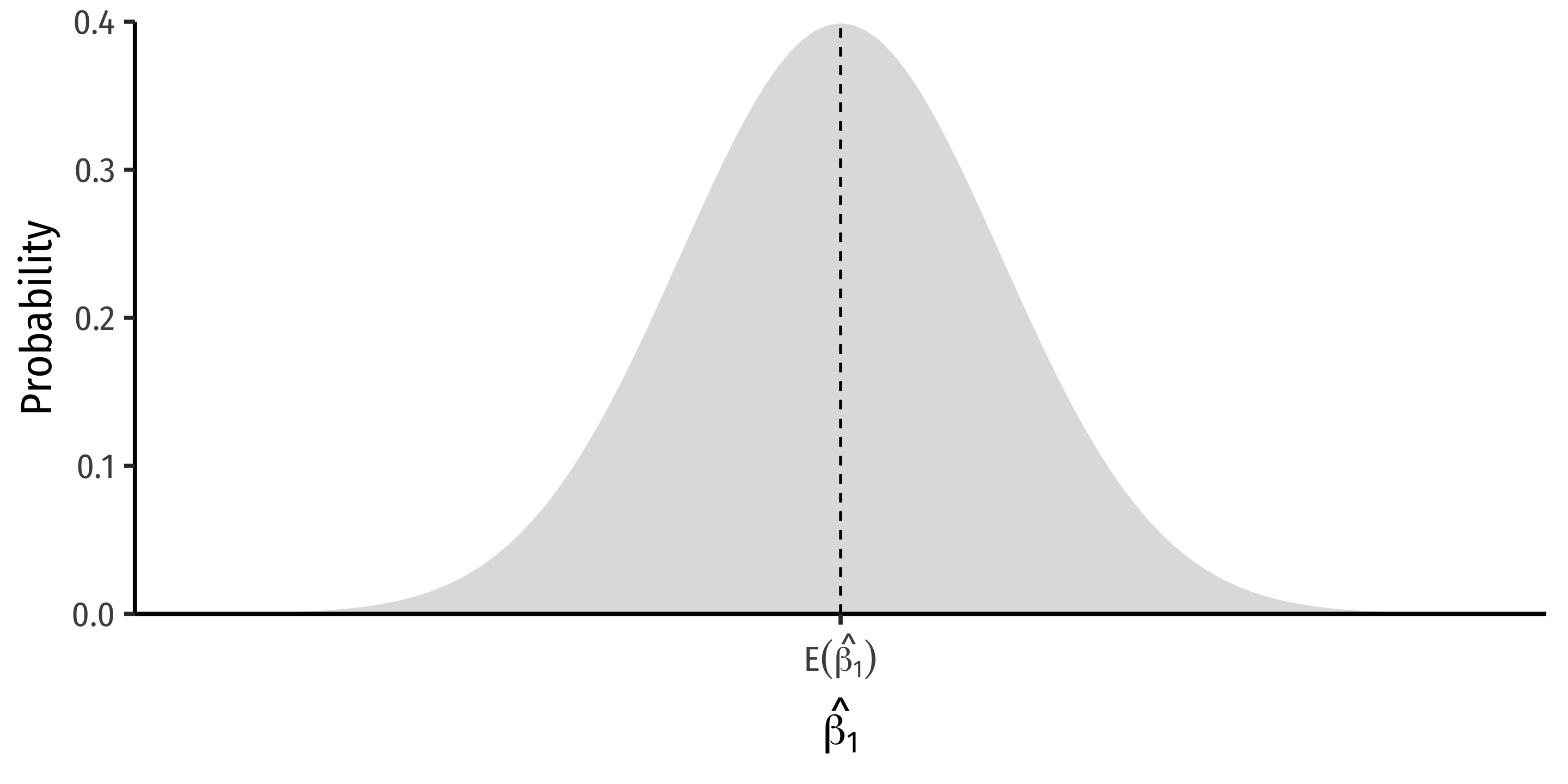
\[\hat{\beta_1} \sim N(\mathbb{E}[\hat{\beta_1}], \sigma_{\hat{\beta_1}})\]

The Sampling Distribution of \(\hat{\beta_1}\) II

\[\hat{\beta_1} \sim N(\mathbb{E}[\hat{\beta_1}], \sigma_{\hat{\beta_1}})\]

• We want to know:

1. \(\mathbb{E}[\hat{\beta_1}]\); what is the center of the distribution? (today)

2. \(\sigma_{\hat{\beta_1}}\); how precise is our estimate? (next class)

Bias and Exogeneity

Assumptions about Errors I

• In order to talk about \(\mathbb{E}[\hat{\beta_1}]\), we need to talk about population \(u\)

• Recall: \(u\) is a random variable, and we can never measure the error term

Assumptions about Errors II

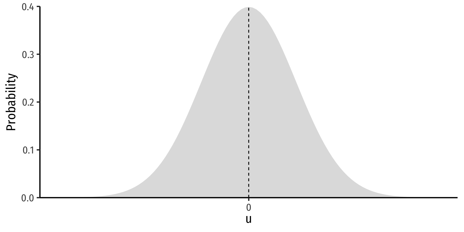
• We make 4 critical assumptions about \(u\):

1. The expected value of the errors is 0

\[\mathbb{E}[u]=0\]

Assumptions about Errors II

• We make 4 critical assumptions about \(u\):

1. The expected value of the errors is 0

\[\mathbb{E}[u]=0\]

2. The variance of the errors over \(X\) is constant:

\[var(u|X)=\sigma^2_{u}\]

Assumptions about Errors II

• We make 4 critical assumptions about \(u\):

1. The expected value of the errors is 0

\[\mathbb{E}[u]=0\]

2. The variance of the errors over \(X\) is constant:

\[var(u|X)=\sigma^2_{u}\]

3. Errors are not correlated across observations:

\[cor(u_i,u_j)=0 \quad \forall i \neq j\]

Assumptions about Errors II

• We make 4 critical assumptions about \(u\):

1. The expected value of the errors is 0

\[\mathbb{E}[u]=0\]

2. The variance of the errors over \(X\) is constant:

\[var(u|X)=\sigma^2_{u}\]

3. Errors are not correlated across observations:

\[cor(u_i,u_j)=0 \quad \forall i \neq j\]

4. There is no correlation between \(X\) and the error term:

\[cor(X, u)=0 \text{ or } E[u|X]=0\]

Assumptions about Errors III

1. The expected value of the errors is 0

\[\mathbb{E}[u]=0\]

2. The variance of the errors over \(X\) is constant:

\[var(u|X)=\sigma^2_{u}\]

• The first two assumptions \(\implies\) errors are i.i.d., drawn from the same distribution with mean 0 and variance \(\sigma^2_{u}\)

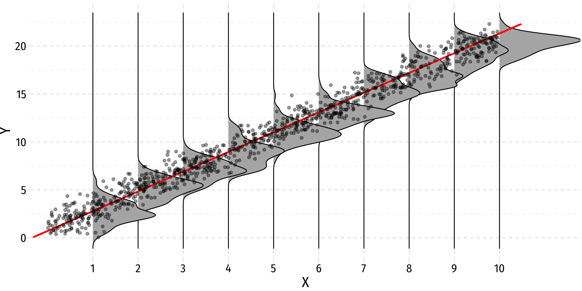
Assumptions about Errors: Homoskedasticity

2. The variance of the errors over \(X\) is constant:

\[var(u|X)=\sigma^2_{u}\]

• Assumption 2 implies that errors are “homoskedastic”: they have the same variance across \(X\)

• Often this assumption is violated: errors may be “heteroskedastic”: they do not have the same variance across \(X\)

• This is a problem for inference, but we have a simple fix for this (next class)

Assumption 3: No Serial Correlation

3. Errors are not correlated across observations:

\[cor(u_i,u_j)=0 \quad \forall i \neq j\]

• For simple cross-sectional data, this is rarely an issue

• Time-series & panel data nearly always contain serial correlation or autocorrelation between errors

• e.g. “this week’s sales look a lot like last week’s sales, which look like…etc”

• There are fixes to deal with autocorrelation (coming much later)

Assumption 4: The Zero Conditional Mean Assumption

• No correlation between \(X\) and the error term:

\[cor(X, u)=0\]

• This is the absolute killer assumption, because it assumes exogeneity

• Often called the Zero Conditional Mean assumption:

\[E[u|X]=0\]

“Does knowing \(X_i\) give any useful information about \(u_i\)?”

• If yes: model is endogenous, biased and not-causal!

Exogeneity and Unbiasedness

• \(\hat{\beta_1}\) is unbiased iff there is no systematic difference, on average, between sample values of \(\hat{\beta_1}\) and true population parameter \(\beta_1\), i.e.

\[E[\hat{\beta_1}]=\beta_1\]

• Does not mean any sample gives us \(\hat{\beta_1}=\beta_1\), only the estimation procedure will, on average, yield the correct value

• Random errors above and below the true value cancel out (so that on average, \(E[\hat{u}|X]=0)\)

Sidenote: Statistical Estimators I

• In statistics, an estimator is a rule for calculating a statistic (about a population parameter)

Example

We want to estimate the average height (H) of U.S. adults (population) and have a random sample of 100 adults.

• Calculate the mean height of our sample \((\bar{H})\) to estimate the true mean height of the population \((\mu_H)\)

• \(\bar{H}\) is an estimator of \(\mu_H\)

• There are many estimators we could use to estimate \(\mu_H\)
  • How about using the first value in our sample: \(H_1\) ?

Sidenote: Statistical Estimators II

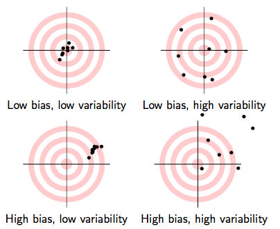
• What makes one estimator (e.g. \(\bar{H}\)) better than another (e.g. \(H_1\))?¹

1. Unbiasedness: does the estimator give us the true parameter on average?

2. Efficiency: an estimator with a smaller variance is better

1. Technically, we also care about consistency: minimizing uncertainty about the correct value. The Law of Large Numbers, similar to CLT, permits this. We don’t need to get too advanced about probability in this class.

Exogeneity and Unbiasedness II

• \(\mathbf{\hat{\beta_1}}\) is the Best Linear Unbiased Estimator (BLUE) estimator of \(\mathbf{\beta_1}\) when \(X\) is exogenous¹

• No systematic difference, on average, between sample values of \(\hat{\beta_1}\) and the true population \(\beta_1\):

\[E[\hat{\beta_1}]=\beta_1\]

• Does not mean that each sample gives us \(\hat{\beta_1}=\beta_1\), only the estimation procedure will, on average, yield the correct value

1. The proof for this is known as the famous Gauss-Markov Theorem. See today’s appendix for a simplified proof.

Exogeneity and Unbiasedness III

• Recall, an exogenous variable \((X)\) is unrelated to other factors affecting \(Y\), i.e.:

\[cor(X,u)=0\]

• Again, this is called the Zero Conditional Mean Assumption

\[E(u|X)=0\]

• For any known value of \(X\), the expected value of \(u\) is 0

• Knowing the value of \(X\) must tell us nothing about the value of \(u\) (anything else relevant to \(Y\) other than \(X\))

• We can then confidently assert causation: \(X \rightarrow Y\)

Endogeneity and Bias

• Nearly all independent variables are endogenous, they are related to the error term \(u\)

\[cor(X,u)\neq 0\]

Example

Suppose we estimate the following relationship:

\[\text{Violent crimes}_t=\beta_0+\beta_1\text{Ice cream sales}_t+u_t\]

• We find \(\hat{\beta_1}>0\)

• Does this mean Ice cream sales \(\rightarrow\) Violent crimes?

Endogeneity and Bias: Takeaways

• The true expected value of \(\hat{\beta_1}\) is actually:¹

\[E[\hat{\beta_1}]=\beta_1+cor(X,u)\frac{\sigma_u}{\sigma_X}\]

1. If \(X\) is exogenous: \(cor(X,u)=0\), we’re just left with \(\beta_1\)

2. The larger \(cor(X,u)\) is, larger bias: \(\left(E[\hat{\beta_1}]-\beta_1 \right)\)

3. We can “sign” the direction of the bias based on \(cor(X,u)\)

• Positive \(cor(X,u)\) overestimates the true \(\beta_1\) \((\hat{\beta_1}\) is too high)
• Negative \(cor(X,u)\) underestimates the true \(\beta_1\) \((\hat{\beta_1}\) is too low)

1. See today’s appendix for proof.

Endogeneity and Bias: Example I

Example

\[wages_i=\beta_0+\beta_1 education_i+u\]

• Is this an accurate reflection of \(education \rightarrow wages\)?

• Does \(E[u|education]=0\)?

• What would \(E[u|education]>0\) mean?

Endogeneity and Bias: Example II

Example

\[\text{per capita cigarette consumption}=\beta_0+\beta_1 \text{State cig tax rate}+u\]

• Is this an accurate reflection of \(taxes \rightarrow consumption\)?

• Does \(E[u|tax]=0\)?

• What would \(E[u|tax]>0\) mean?