2.6 — Inference for Regression
ECON 480 • Econometrics • Fall 2022
Dr. Ryan Safner
Associate Professor of Economics
safner@hood.edu
ryansafner/metricsF22
metricsF22.classes.ryansafner.com
Contents
Why Uncertainty Matters
Recall: Two Big Problems with Data
- We use econometrics to identify causal relationships & make inferences about them:
- Problem for identification: endogeneity
- X is exogenous if cor(x,u)=0
- X is endogenous if cor(x,u)≠0
- Problem for inference: randomness
- Data is random due to natural sampling variation
- Taking one sample of a population will yield slightly different information than another sample of the same population


Distributions of the OLS Estimators
Yi=β0+β1Xi+ui
OLS estimators (^β0 and ^β1) are computed from a finite (specific) sample of data
Our OLS model contains 2 sources of randomness:
- Modeled randomness: population ui includes all factors affecting Y other than X
- different samples will have different values of those other factors (ui)
- Sampling randomness: different samples will generate different OLS estimators
- Thus, ^β0,^β1 are also random variables, with their own sampling distribution
The Two Problems: Where We’re Heading…Ultimately
Sample statistical inference→ Population causal indentification→ Unobserved Parameters
- We want to identify causal relationships between population variables
- Logically first thing to consider
- Endogeneity problem
- We’ll use sample statistics to infer something about population parameters
- In practice, we’ll only ever have a finite sample distribution of data
- We don’t know the population distribution of data
- Randomness problem
Why Sample vs. Population Matters
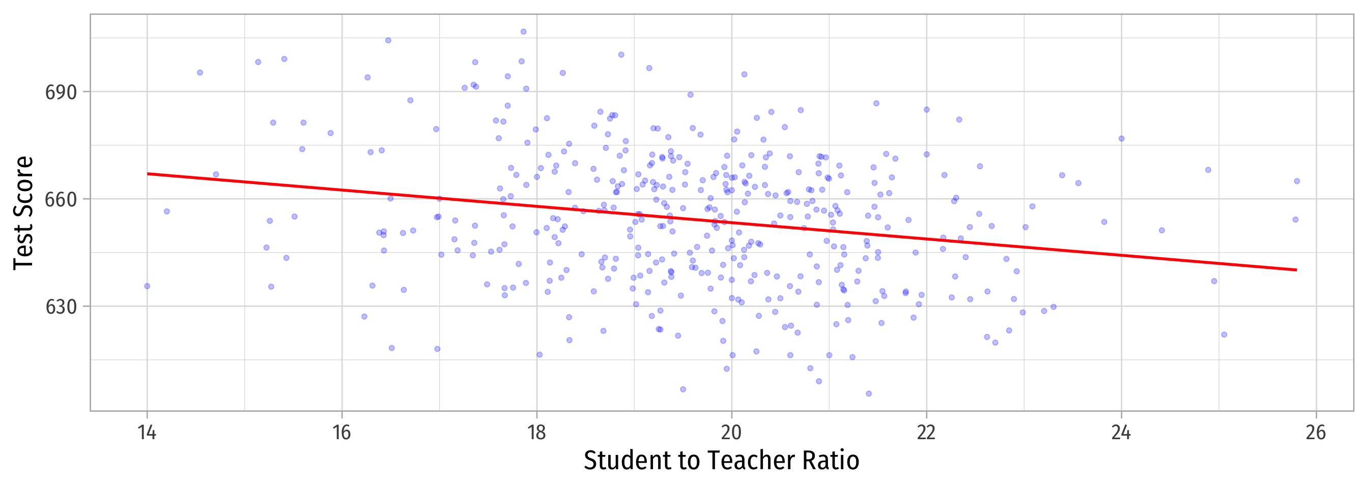
Population relationship
Yi=698.93+−2.28Xi+ui
Yi=β0+β1Xi+ui
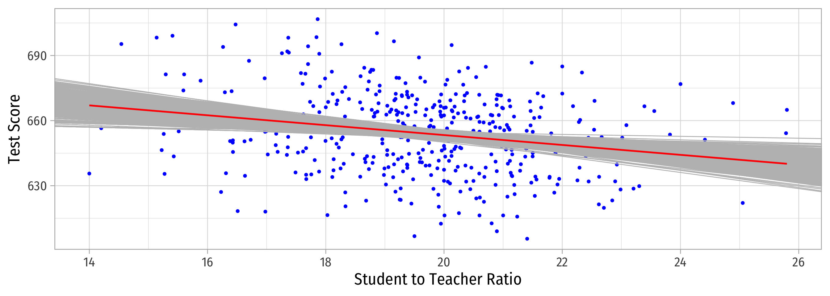
Why Sample vs. Population Matters
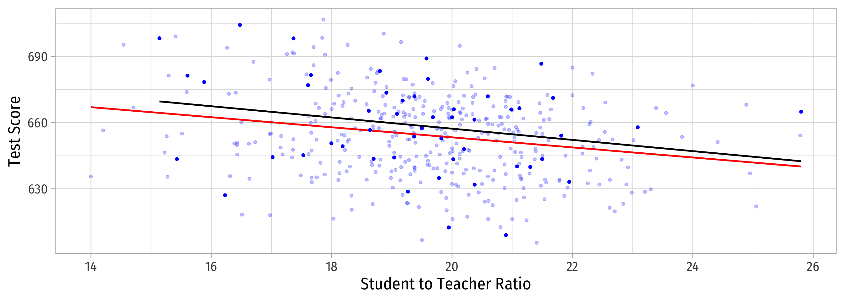
Sample 1: 50 random observations
Population relationship
Yi=698.93+−2.28Xi+ui
Sample relationship
ˆYi=708.12+−2.54Xi
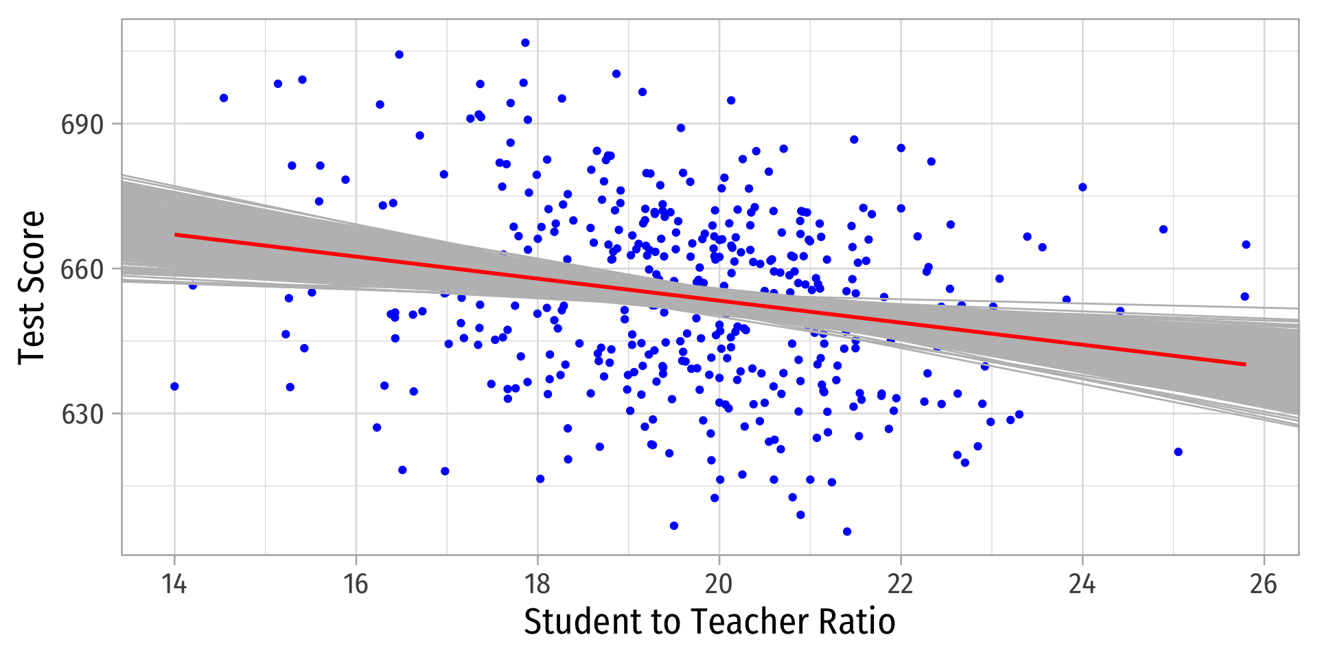
Why Sample vs. Population Matters
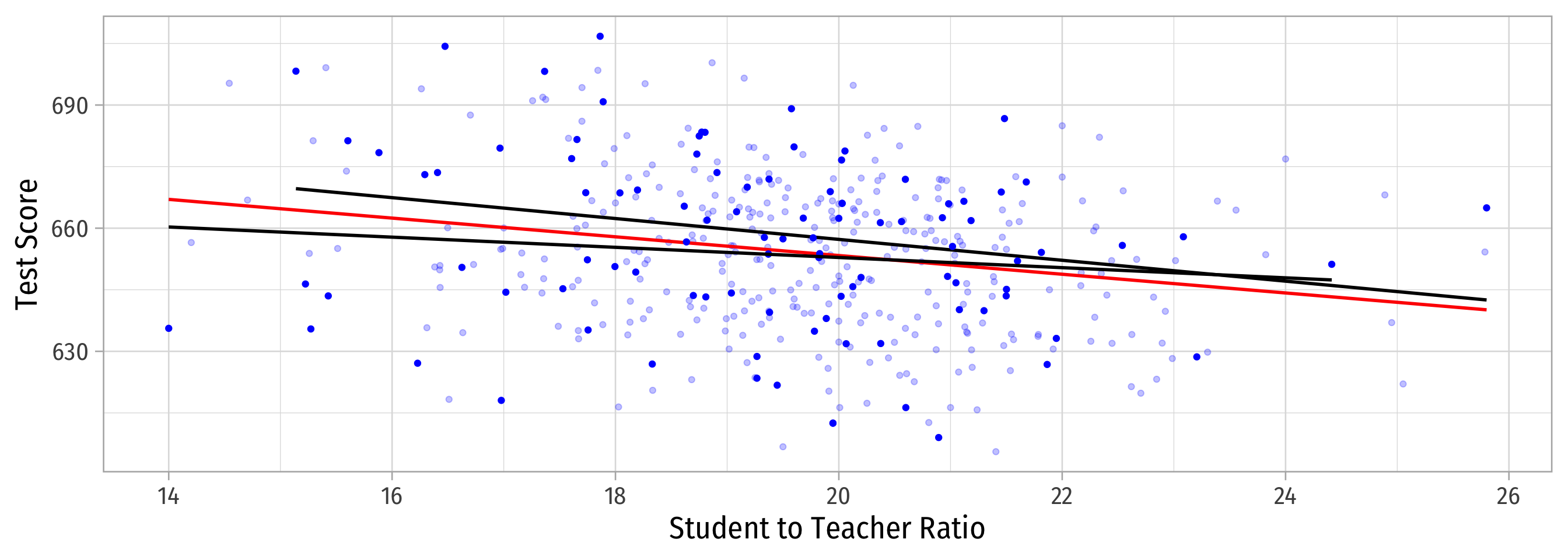
Sample 2: 50 random individuals
Population relationship
Yi=698.93+−2.28Xi+ui
Sample relationship
ˆYi=708.12+−2.54Xi
Why Sample vs. Population Matters
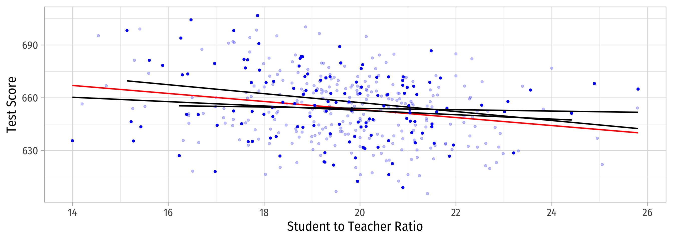
Sample 3: 50 random individuals
Population relationship
Yi=698.93+−2.28Xi+ui
Sample relationship
ˆYi=708.12+−2.54Xi
Why Sample vs. Population Matters
Let’s repeat this process 10,000 times!
This exercise is called a (Monte Carlo) simulation
- I’ll show you how to do this next class with the
inferpackage
- I’ll show you how to do this next class with the
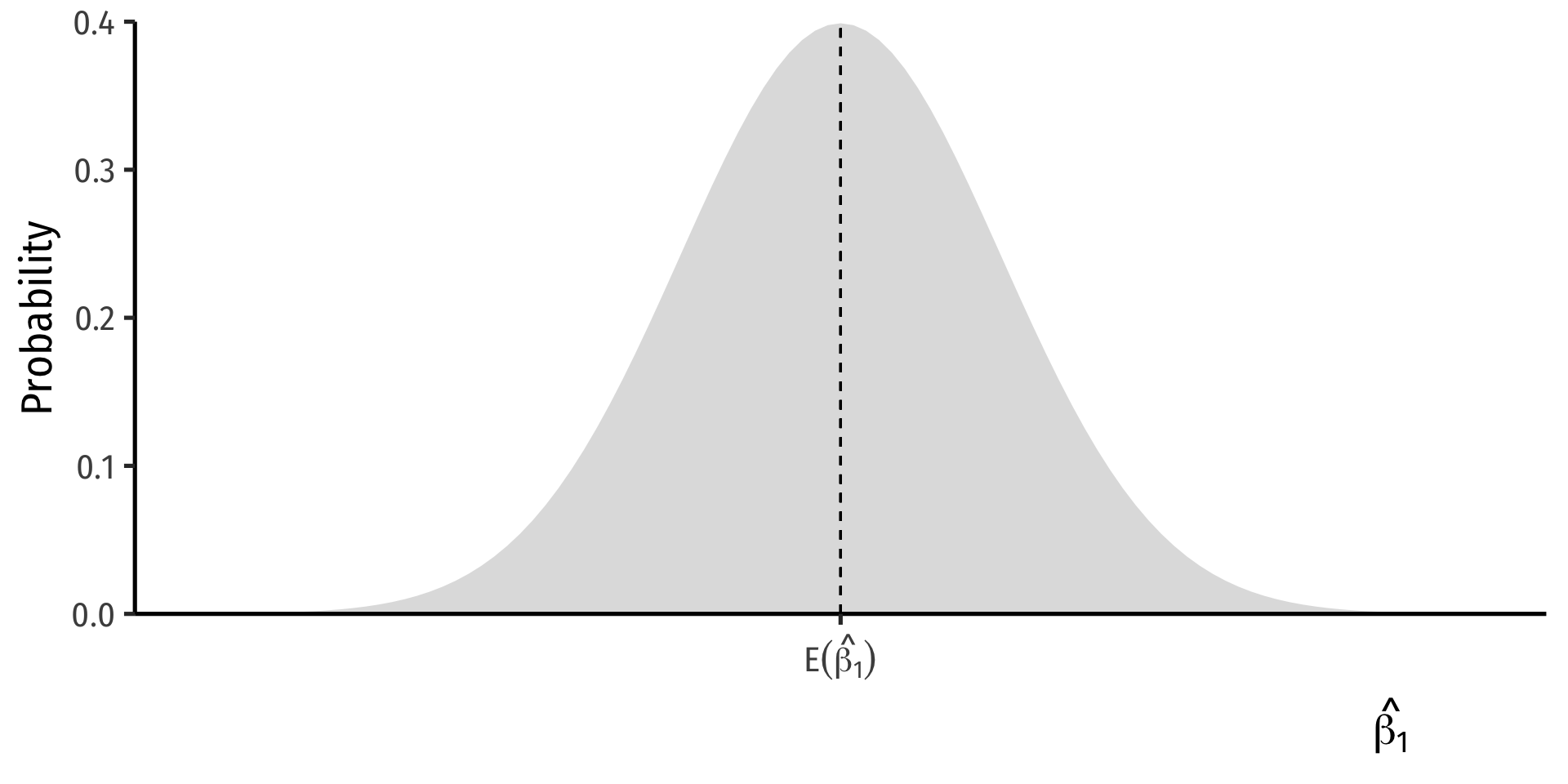
Why Sample vs. Population Matters
- On average, estimated regression lines from (hypothetical) samples provide an unbiased estimate of true population regression line
E[ˆβ1]=β1
But, any individual estimate can miss the mark
This leads to uncertainty about our estimated regression line
- We only have 1 sample in reality!
- This is why we care about the standard error of our line: se(^β1)!
Confidence Intervals
Statistical Inference
Sample statistical inference→ Population causal indentification→ Unobserved Parameters
- We want to start inferring what the true population regression model is, using our estimated regression model from our sample
^Yi=^β0+^β1X🤞 hopefully 🤞→Yi=β0+β1X+ui
- We can’t yet make causal inferences about whether/how X causes Y
- coming after the midterm!
Estimation and Statistical Inference
Our problem with uncertainty is we don’t know whether our sample estimate is close or far from the unknown population parameter
But we can use our errors to learn how well our model statistics likely estimate the true parameters
Use ^β1 and its standard error, se(^β1) for statistical inference about true β1
We have two options…
Estimation and Statistical Inference

- Use our ^β1 & se(^β1) to determine if statistically significant evidence to reject a hypothesized β1

- Use our ^β1 & se(^β1) to create a range of values that gives us a good chance of capturing the true β1
Accuracy vs. Precision

Generating Confidence Intervals
- We can generate our confidence interval by generating a “bootstrap” sampling distribution:
- Take our sample data and resample it many times by selecting random observations and then replacing them
- This allows us to approximate the sampling distribution of ^β1 by simulation!

Confidence Intervals Using the infer Package
Confidence Intervals Using the infer Package I
Confidence Intervals Using the infer Package II

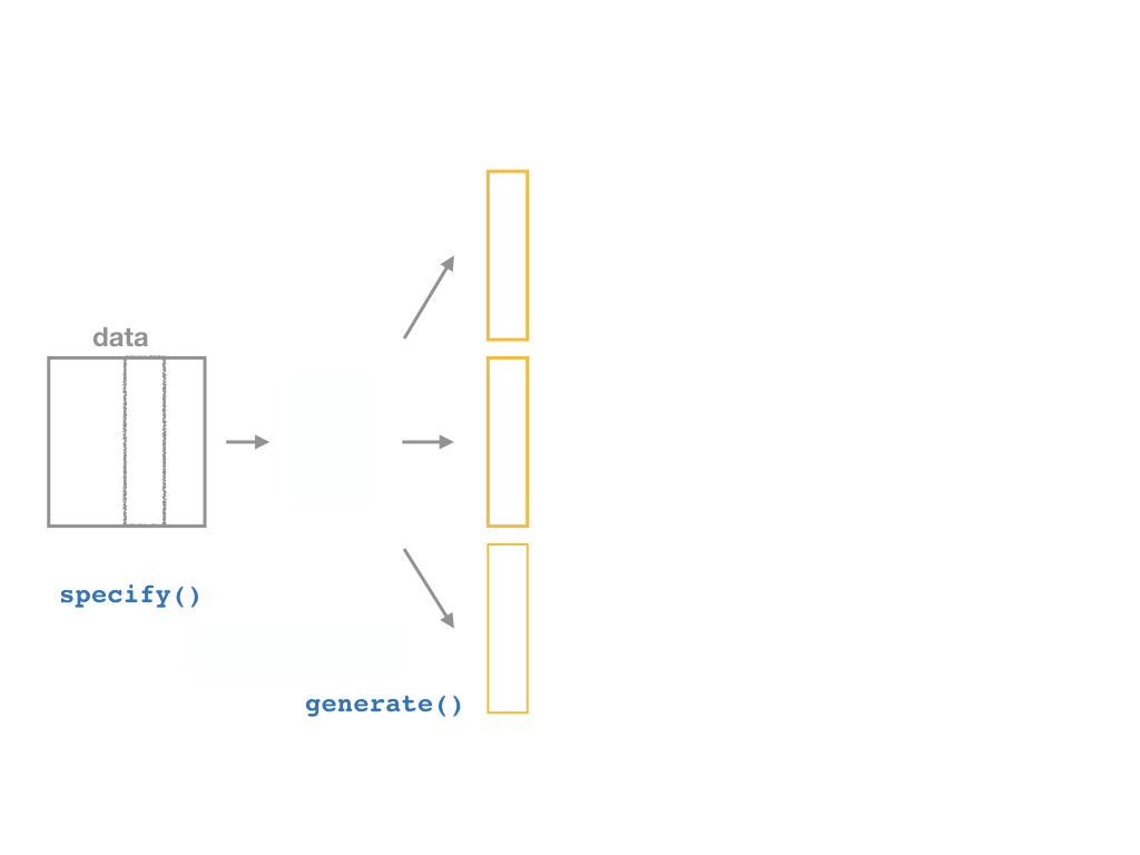
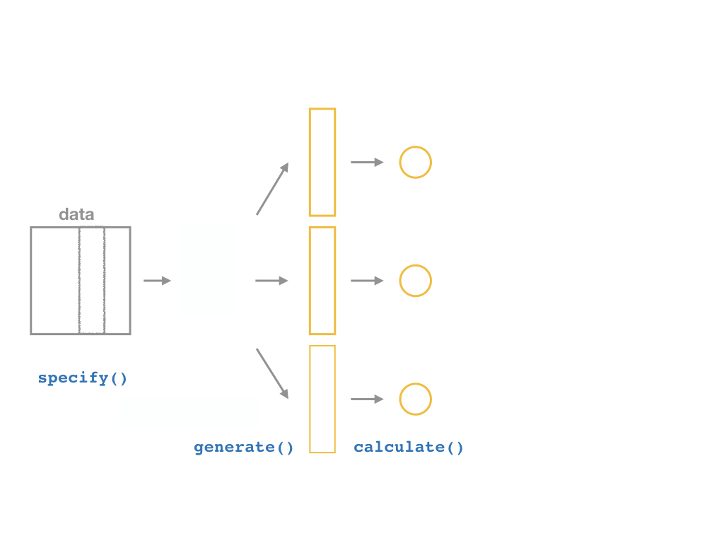
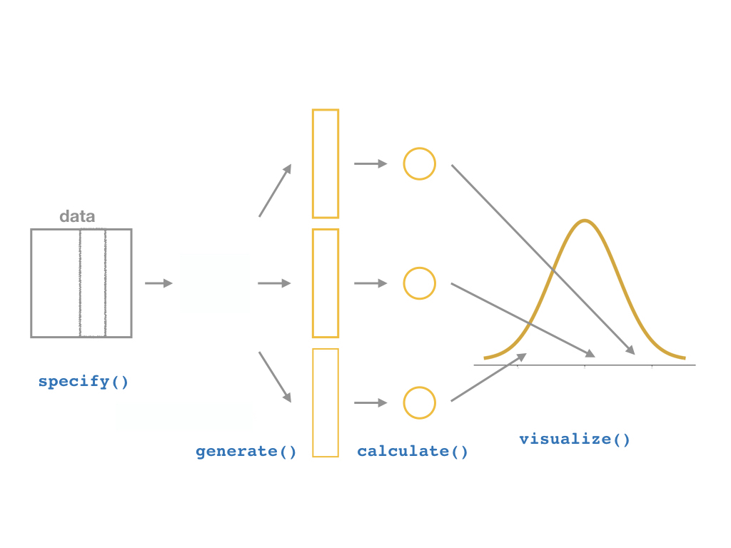
inferallows you to run through these steps manually to understand the process:
specify()a modelgenerate()a bootstrap distributioncalculate()the confidence intervalvisualize()with a histogram (optional)
Confidence Intervals Using the infer Package III

Confidence Intervals Using the infer Package III
Confidence Intervals Using the infer Package III
Confidence Intervals Using the infer Package III
Confidence Intervals Using the infer Package III
Bootstrapping
Our Sample
| ABCDEFGHIJ0123456789 |
term <chr> | estimate <dbl> | std.error <dbl> | statistic <dbl> | p.value <dbl> |
|---|---|---|---|---|
| (Intercept) | 698.932952 | 9.4674914 | 73.824514 | 6.569925e-242 |
| str | -2.279808 | 0.4798256 | -4.751327 | 2.783307e-06 |
Another “Sample”
| ABCDEFGHIJ0123456789 |
term <chr> | estimate <dbl> | std.error <dbl> | statistic <dbl> | p.value <dbl> |
|---|---|---|---|---|
| (Intercept) | 671.5164920 | 8.9597708 | 74.947954 | 1.853313e-244 |
| str | -0.9595986 | 0.4521103 | -2.122488 | 3.438415e-02 |
👆 Bootstrapped from Our Sample
- Now we want to do this 1,000 times to simulate the (unknown) sampling distribution of ^β1
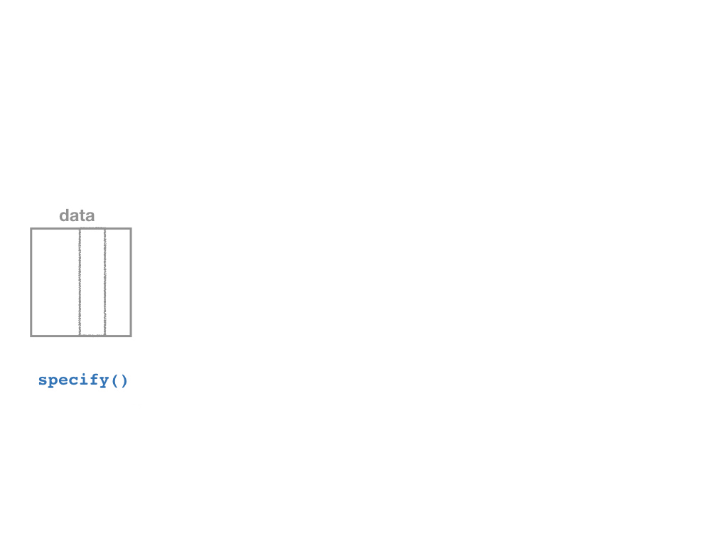
The infer Pipeline: specify()
The infer Pipeline: specify()
Specify
data %>%
specify(y ~ x)
- Take our data and pipe it into the
specify()function, which is essentially alm()function for regression (for our purposes)
The infer Pipeline: generate()
The infer Pipeline: generate()
The infer Pipeline: generate()
Specify
Generate
%>% generate(reps = n, type = "bootstrap")
Now the magic starts, as we run a number of simulated samples
Set the number of
repsand settypeto"bootstrap"
replicate: the “sample” number (1-1000)creates
xandyvalues (data points)
The infer Pipeline: calculate()
The infer Pipeline: calculate()
The infer Pipeline: calculate()
The infer Pipeline: calculate()
Specify
Generate
Calculate
%>% calculate(stat = "slope")
Confidence Interval
- A 95% confidence interval is the middle 95% of the sampling distribution
Confidence Interval
- A 95% confidence interval is the middle 95% of the sampling distribution

The infer Pipeline: get_confidence_interval()
Specify
Generate
Calculate
Get Confidence Interval
%>% get_confidence_interval()
Broom Can Estimate a Confidence Interval
| ABCDEFGHIJ0123456789 |
term <chr> | estimate <dbl> | std.error <dbl> | statistic <dbl> | p.value <dbl> | |
|---|---|---|---|---|---|
| (Intercept) | 698.932952 | 9.4674914 | 73.824514 | 6.569925e-242 | |
| str | -2.279808 | 0.4798256 | -4.751327 | 2.783307e-06 |
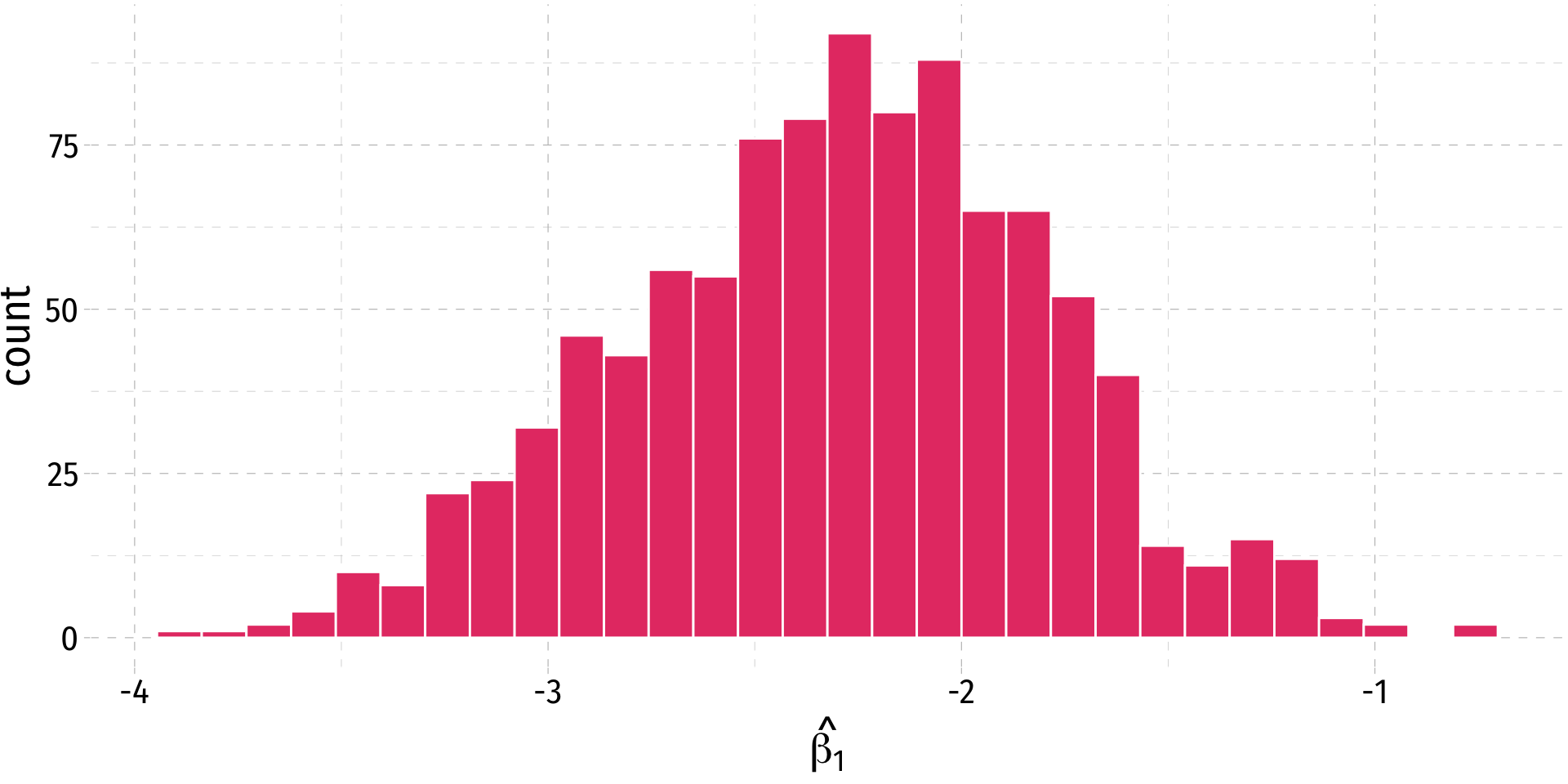
The infer Pipeline: visualize()

The infer Pipeline: visualize()
Specify
Generate
Calculate
Visualize
%>% visualize()

Confidence Intervals, Theory
Confidence Intervals, Theory
- In general, a confidence interval (CI) takes a point estimate and extrapolates it within some margin of error (MOE):
([ estimate - MOE ], [ estimate + MOE ])
- The main question is, how confident do we want to be that our interval contains the true parameter?
- Larger confidence level, larger margin of error (and thus larger interval)
Confidence Intervals, Theory
- (1−α) is the confidence level of our confidence interval
- α is the “significance level” that we use in hypothesis testing
- α= probability that the true parameter is not contained within our interval
- Typical levels: 90%, 95%, 99%
- 95% is especially common, α=0.05
Confidence Levels
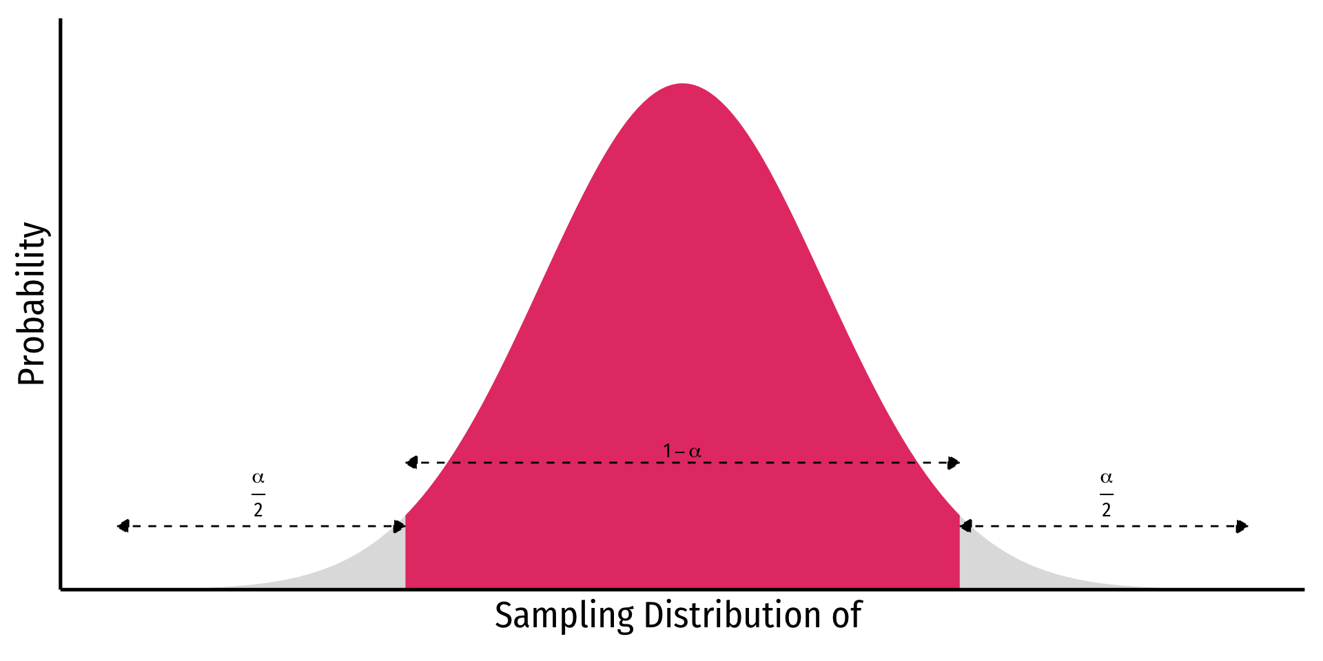
Depending on our confidence level, we are essentially looking for the middle (1−α)% of the sampling distribution
This puts α in the tails; α2 in each tail
Confidence Levels and the Empirical Rule
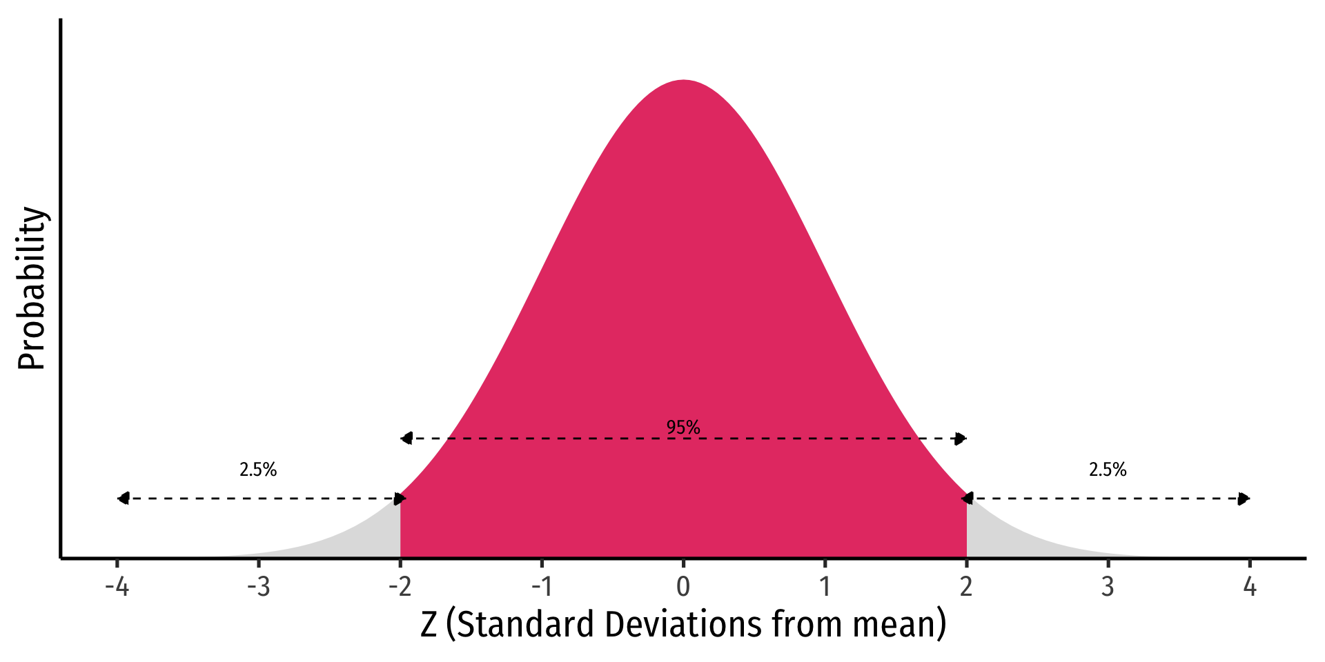
Recall the 68-95-99.7% empirical rule for (standard) normal distributions!1
95% of data falls within 2 standard deviations of the mean
Thus, in 95% of samples, the true parameter is likely to fall within about 2 standard deviations of the sample estimate
Interpretting Confidence Intervals
- So our confidence interval for our slope is (-3.22, -1.33), what does this mean again?
❌ 95% of the time, the true effect of class size on test score will be between -3.22 and -1.33
❌ We are 95% confident that a randomly selected school district will have an effect of class size on test score between -3.22 and -1.33
❌ The effect of class size on test score is -2.28 95% of the time.
✅ We are 95% confident that in similarly constructed samples, the true effect is between -3.22 and -1.33
Estimating in R
base Rdoesn’t show confidence intervals in thelm summary()output, need theconfintcommand
                2.5 %     97.5 %
(Intercept) 680.32313 717.542779
str          -3.22298  -1.336637
Estimating with broom
broom’stidy()command can include confidence intervals
| ABCDEFGHIJ0123456789 |
term <chr> | estimate <dbl> | std.error <dbl> | statistic <dbl> | p.value <dbl> | |
|---|---|---|---|---|---|
| (Intercept) | 698.932952 | 9.4674914 | 73.824514 | 6.569925e-242 | |
| str | -2.279808 | 0.4798256 | -4.751327 | 2.783307e-06 |

