Estimation and Hypothesis Testing I
- We want to test if our estimates are statistically significant and they describe the population
- this is the “bread and butter” of using inferential statistics
Examples
- Does reducing class size improve test scores?
- Do more years of education increase your wages?
- Is the gender wage gap between men and women 23%?

All modern science is built upon statistical hypothesis testing, so understand it well
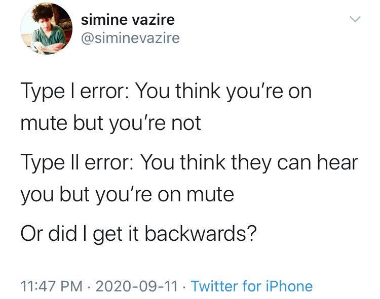
Type I and Type II Errors III
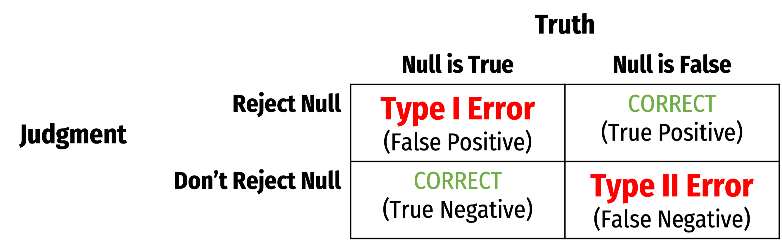
- Depending on context, committing one type of error may be more serious than the other
Type I and Type II Errors IV
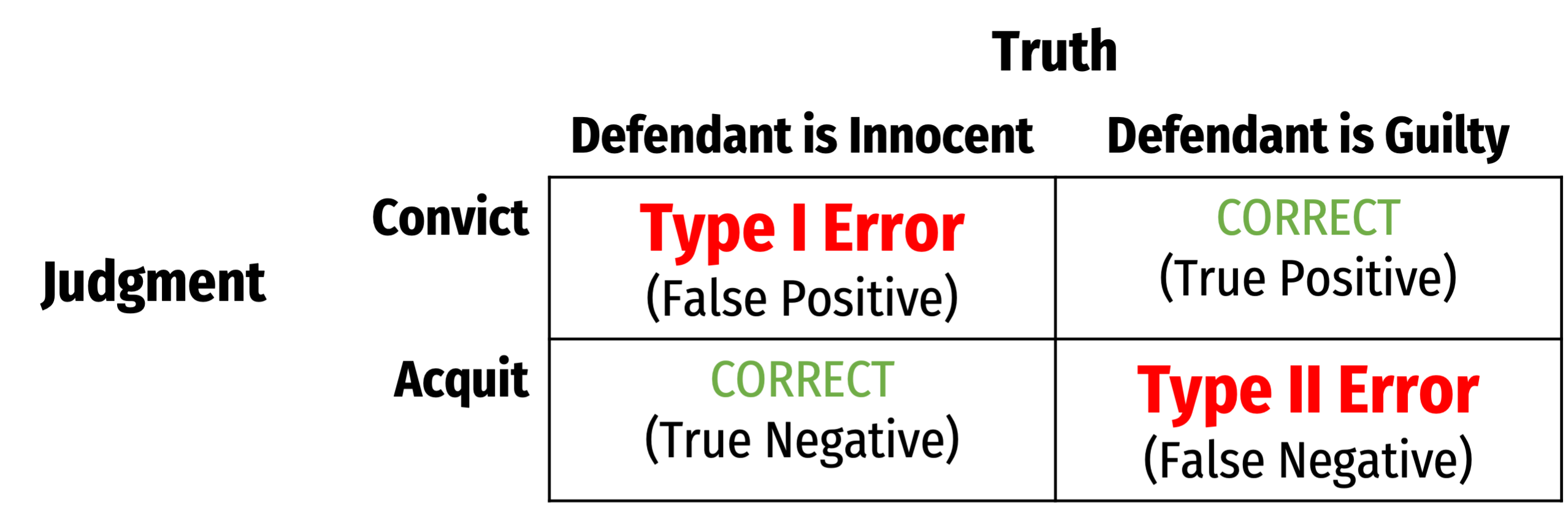
- Anglo-American common law presumes defendant is innocent: \(H_0\)
- Jury judges whether the evidence presented against the defendant is plausible assuming the defendant were in fact innocent
- If highly improbable (beyond a “reasonable doubt”): sufficient evidence to reject \(H_0\) and convict
Type I and Type II Errors V
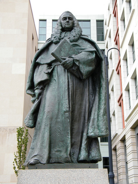
William Blackstone
(1723-1780)
“It is better that ten guilty persons escape than that one innocent suffer.”
- Type I error is worse than a Type II error in law!
Blackstone, William, 1765-1770, Commentaries on the Laws of England
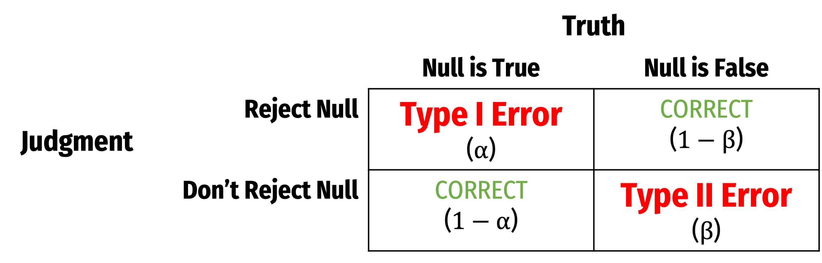
Type I and Type II Errors VI
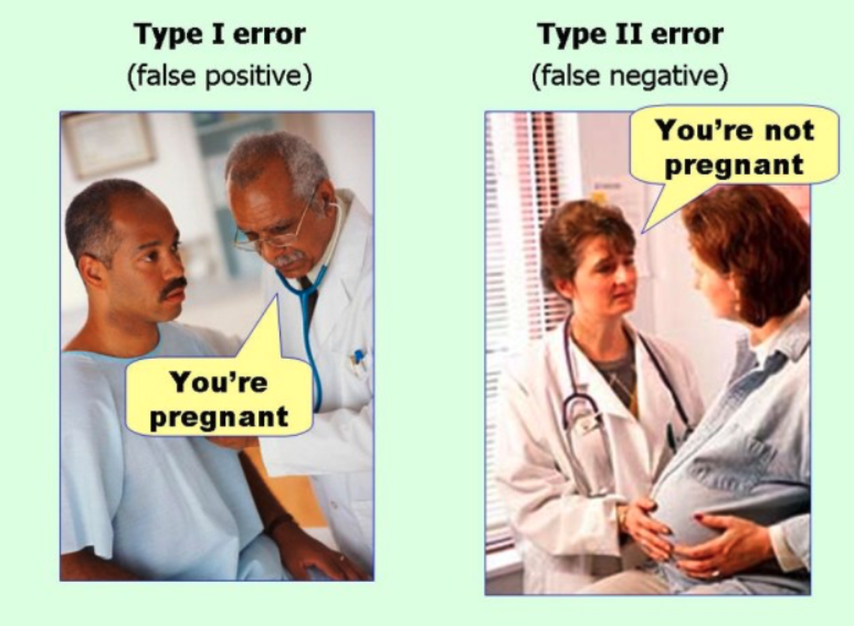
Type I and Type II Errors VII
\(\alpha\) and \(\beta\)
Hypothesis Testing and the Philosophy of Science I

Sir Ronald A. Fisher
(1890-1962)
“The null hypothesis is never proved or established, but is possibly disproved, in the course of experimentation. Every experiment may be said to exist only in order to give the facts a chance of disproving the null hypothesis.”
Fisher, R.A., 1931, The Design of Experiments
Hypothesis Testing and the Philosophy of Science II
Modern philosophy of science is largely based off of hypothesis testing and falsifiability, which form the “Scientific Method”1
For something to be “scientific”, it must be falsifiable, or at least testable (at least in principle)
Hypotheses can be corroborated with evidence, but always tentative until falsified by data in suggesting an alternative hypothesis
“All swans are white” is a hypothesis rejected upon discovery of a single black swan

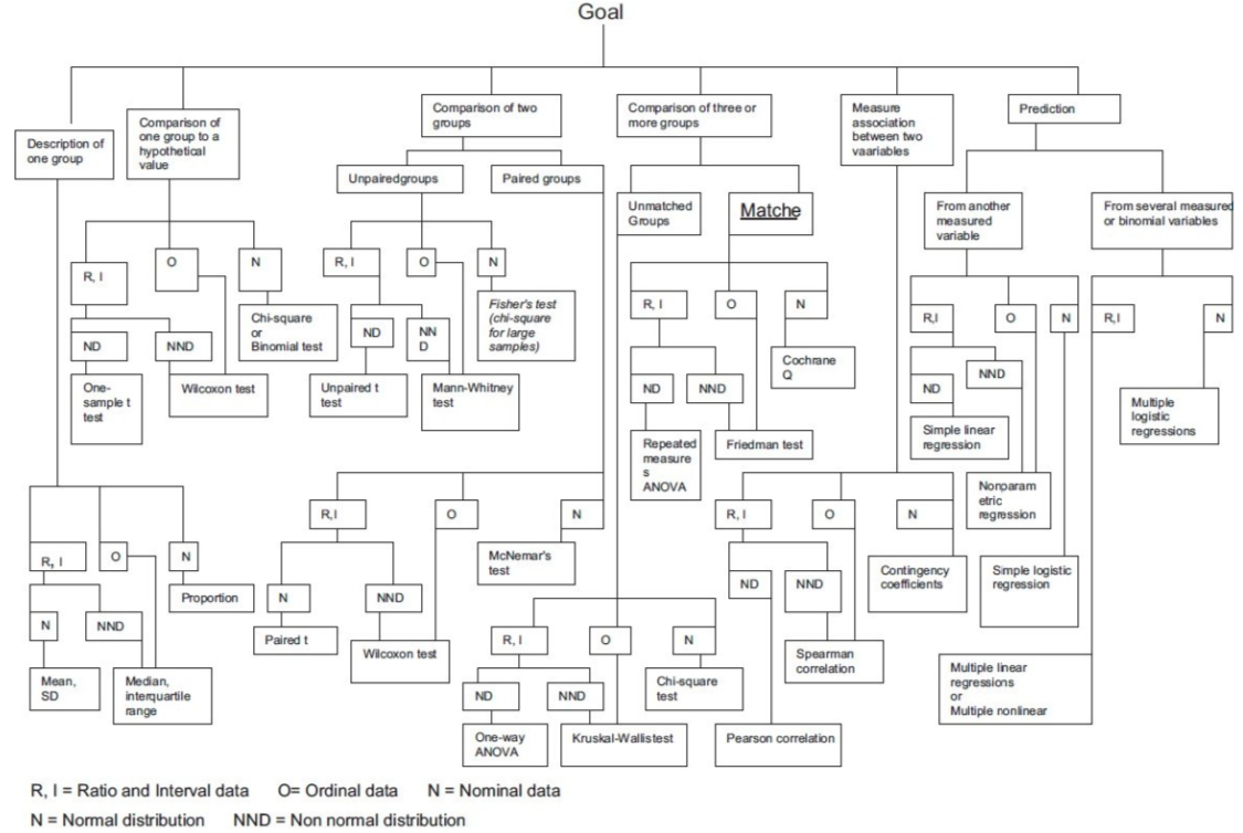
Hypothesis Testing: Which Test? II
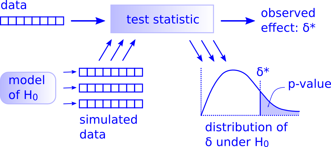
Elements of a Hypothesis Test
Hypothesis Testing with the infer Package II

Hypothesis Testing with the infer Package II

Hypothesis Testing with the infer Package II
Hypothesis Testing with the infer Package II
Hypothesis Testing with the infer Package II
Hypothesis Testing with the infer Package II
Theory-Based Inference: Critical Values of Test Statistic

Imagine a Null World, where \(H_0\) is True

Our world, and a world where \(\beta_1=0\) by assumption.
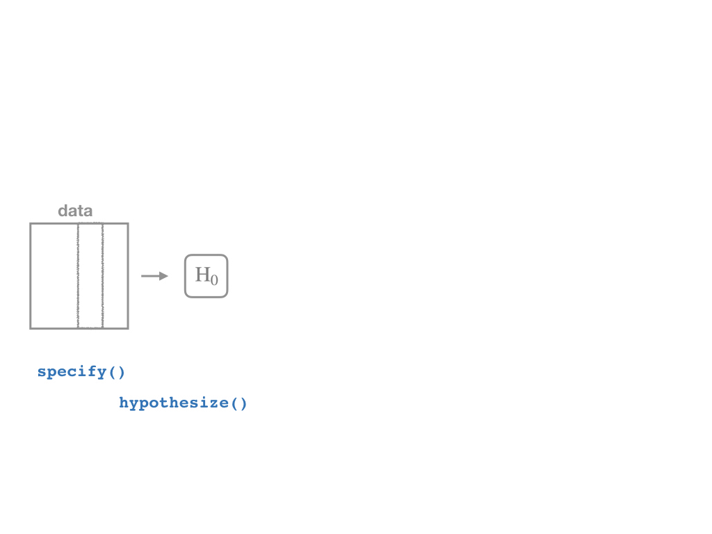
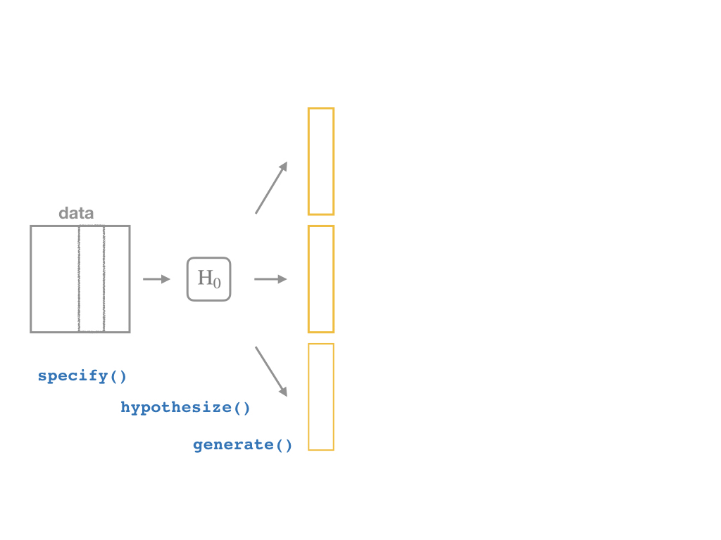
The infer Pipeline: specify()
The infer Pipeline: hypothesize()
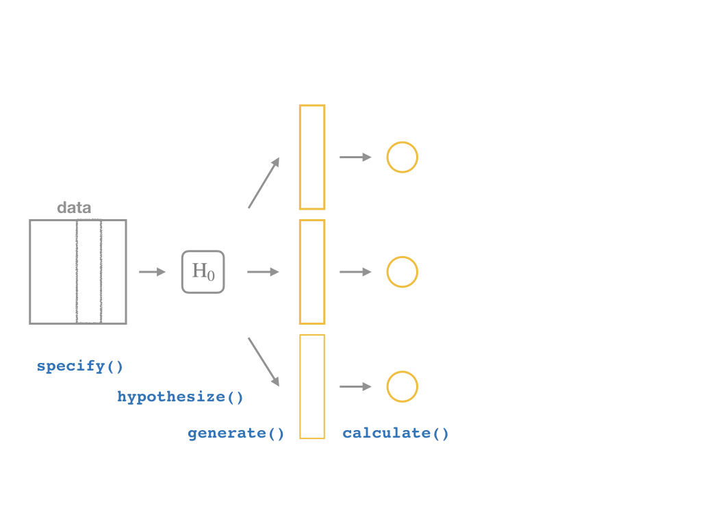
The infer Pipeline: generate()
The infer Pipeline: calculate()
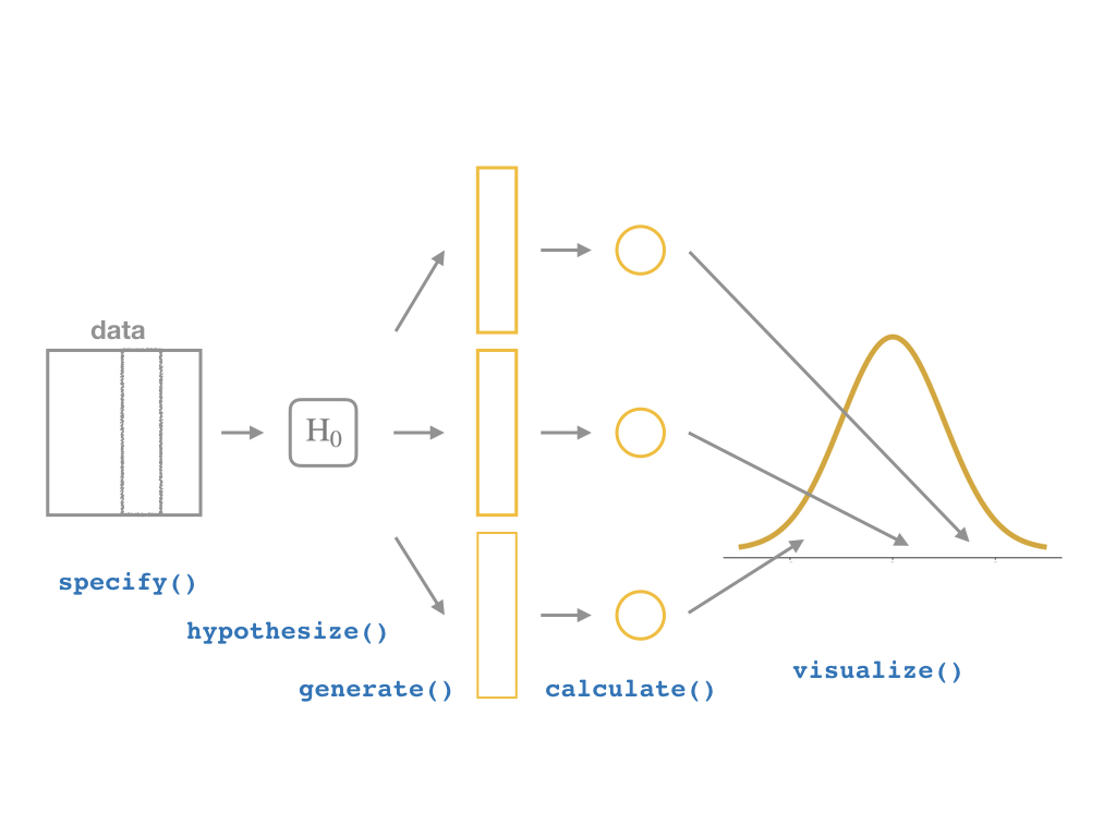
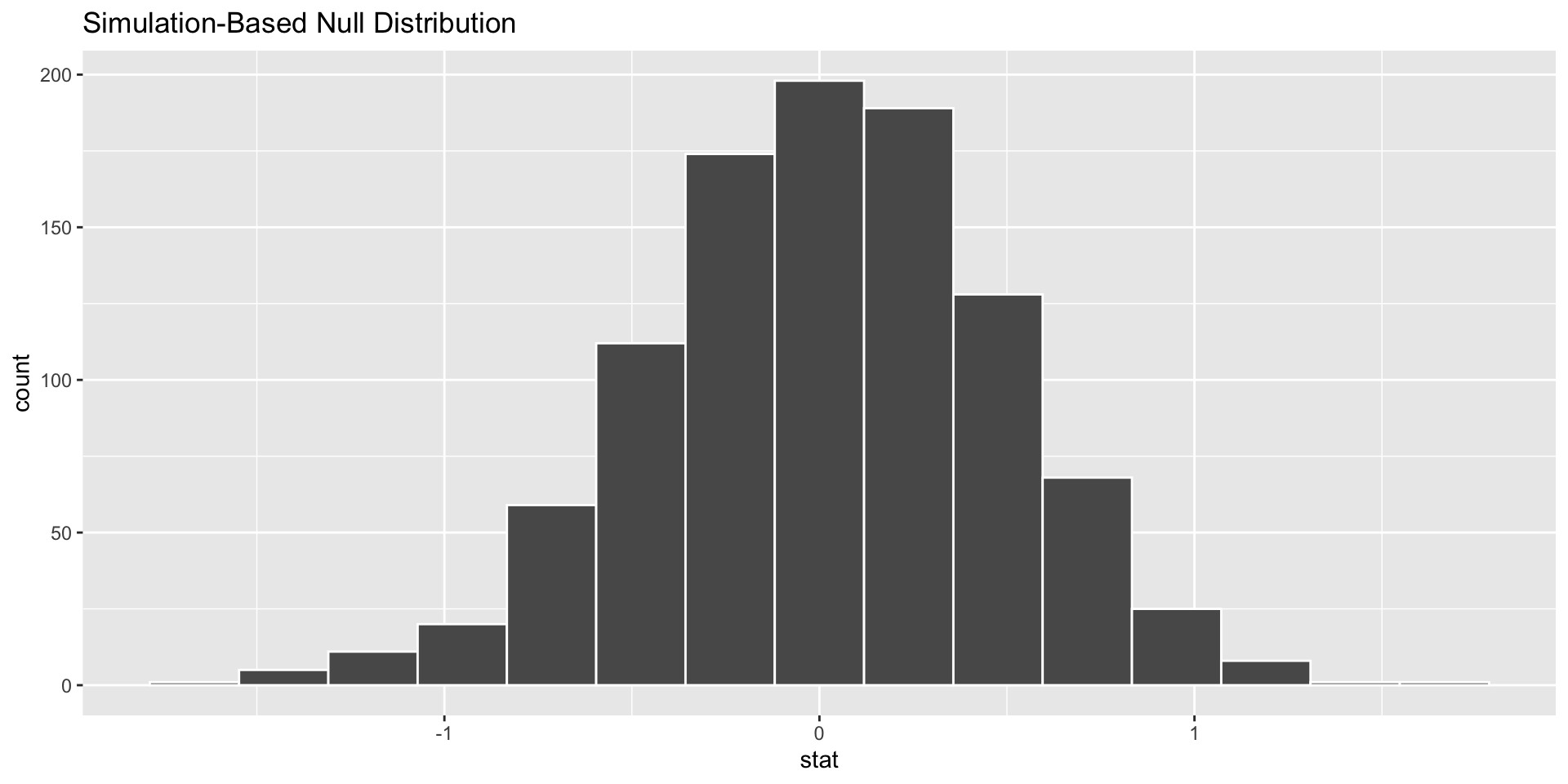
The infer Pipeline: visualize()
The infer Pipeline: visualize()
data %>%
specify(y ~ x) %>%
hypothesize(null = "independence") %>%
generate(reps = n, type = "permute") %>%
calculate(stat = "slope") %>%
visualize()
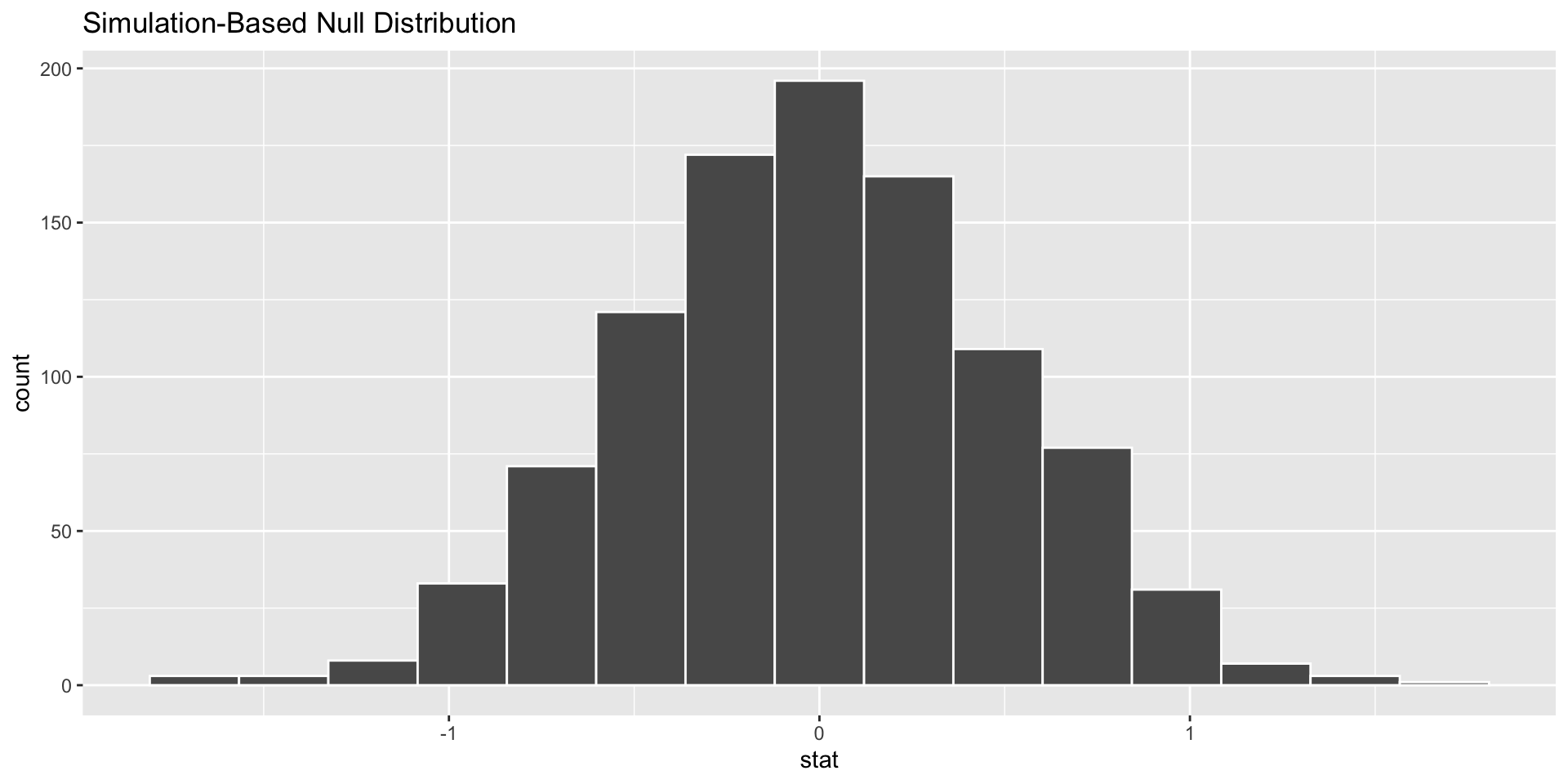
The infer Pipeline: visualize()
data %>%
specify(y ~ x) %>%
hypothesize(null = "independence") %>%
generate(reps = n, type = "permute") %>%
calculate(stat = "slope") %>%
visualize()
The infer Pipeline: visualize()
data %>%
specify(y ~ x) %>%
hypothesize(null = "independence") %>%
generate(reps = n, type = "permute") %>%
calculate(stat = "slope") %>%
visualize() + shade_p_value()

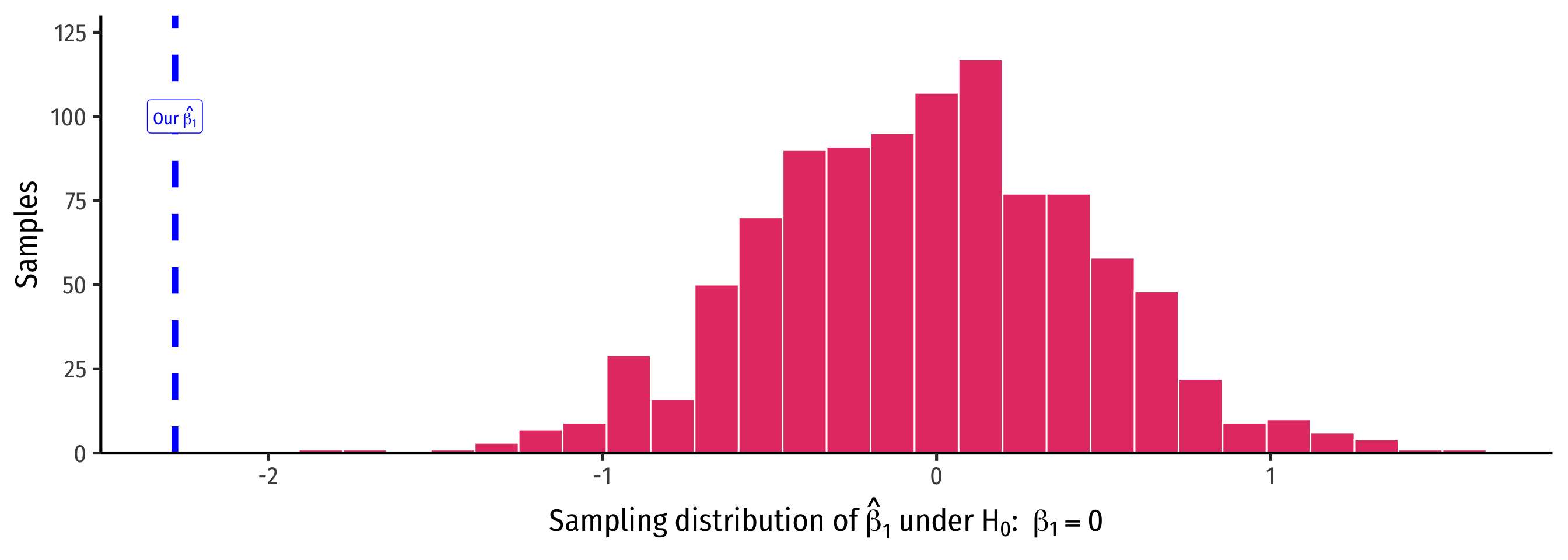
visualize() is Just a Wrapper for ggplot
# infer
ca_school %>%
specify(testscr ~ str) %>%
hypothesize(null = "independence") %>%
generate(reps = 1000,
type = "permute") %>%
calculate(stat = "slope") %>%
# pipe into ggplot
ggplot(data = )+
aes(x = stat)+
geom_histogram(color="white", fill="#e64173")+
geom_vline(xintercept = our_slope,
color = "blue",
size = 2,
linetype = "dashed")+
annotate(geom = "label",
x = -2.28,
y = 100,
label = expression(paste("Our ", hat(beta[1]))),
color = "blue")+
scale_y_continuous(lim=c(0,130),
expand = c(0,0))+
labs(x = expression(paste("Sampling distribution of ", hat(beta)[1], " under ", H[0], ": ", beta[1]==0)),
y = "Samples")+
theme_classic(base_family = "Fira Sans Condensed",
base_size=20)What R Does: Theory-Based Statistical Inference I
R does things the old-fashioned way, using a theoretical null distribution instead of simulating one
A t-distribution with \(n-k-1\) df1
Calculate a \(t\)-statistic for \(\hat{\beta_1}\):
\[\text{test statistic} = \frac{\text{estimate} - \text{null hypothesis}}{\text{standard error of estimate}}\]

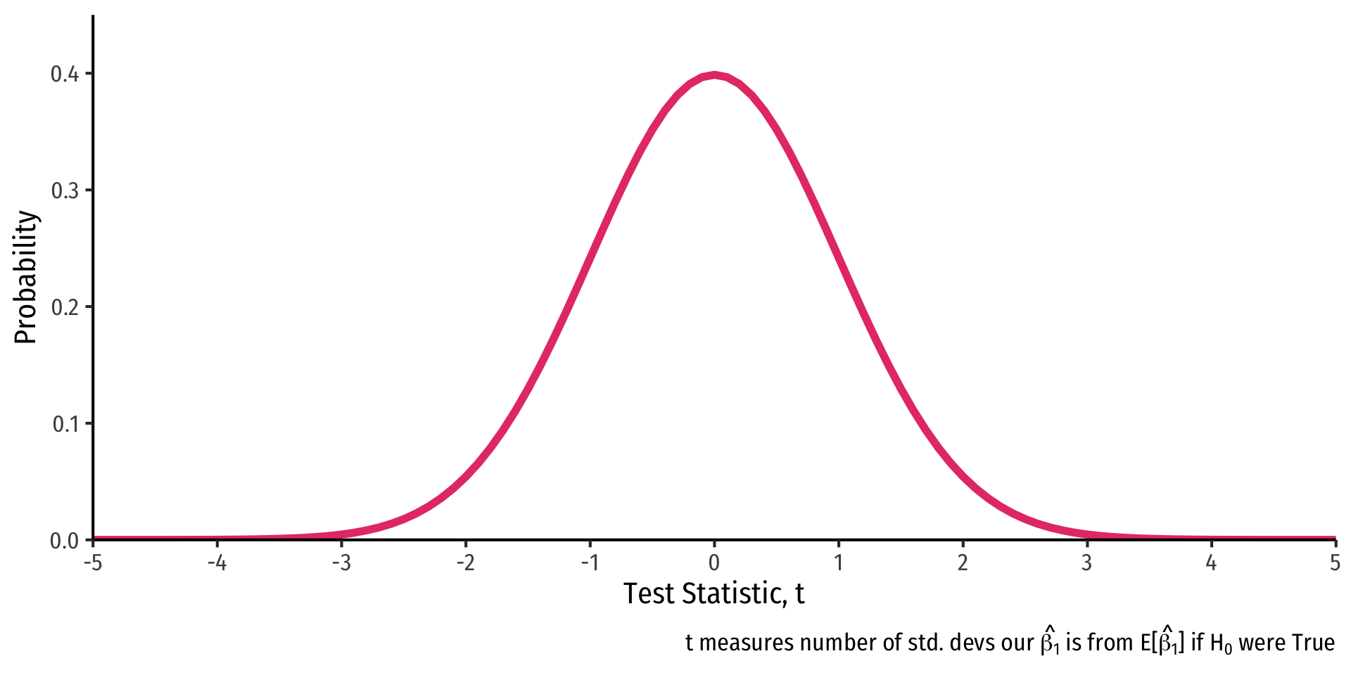
What R Does: Theory-Based Statistical Inference II
\[\text{test statistic} = \frac{\text{estimate} - \text{null hypothesis}}{\text{standard error of estimate}}\]
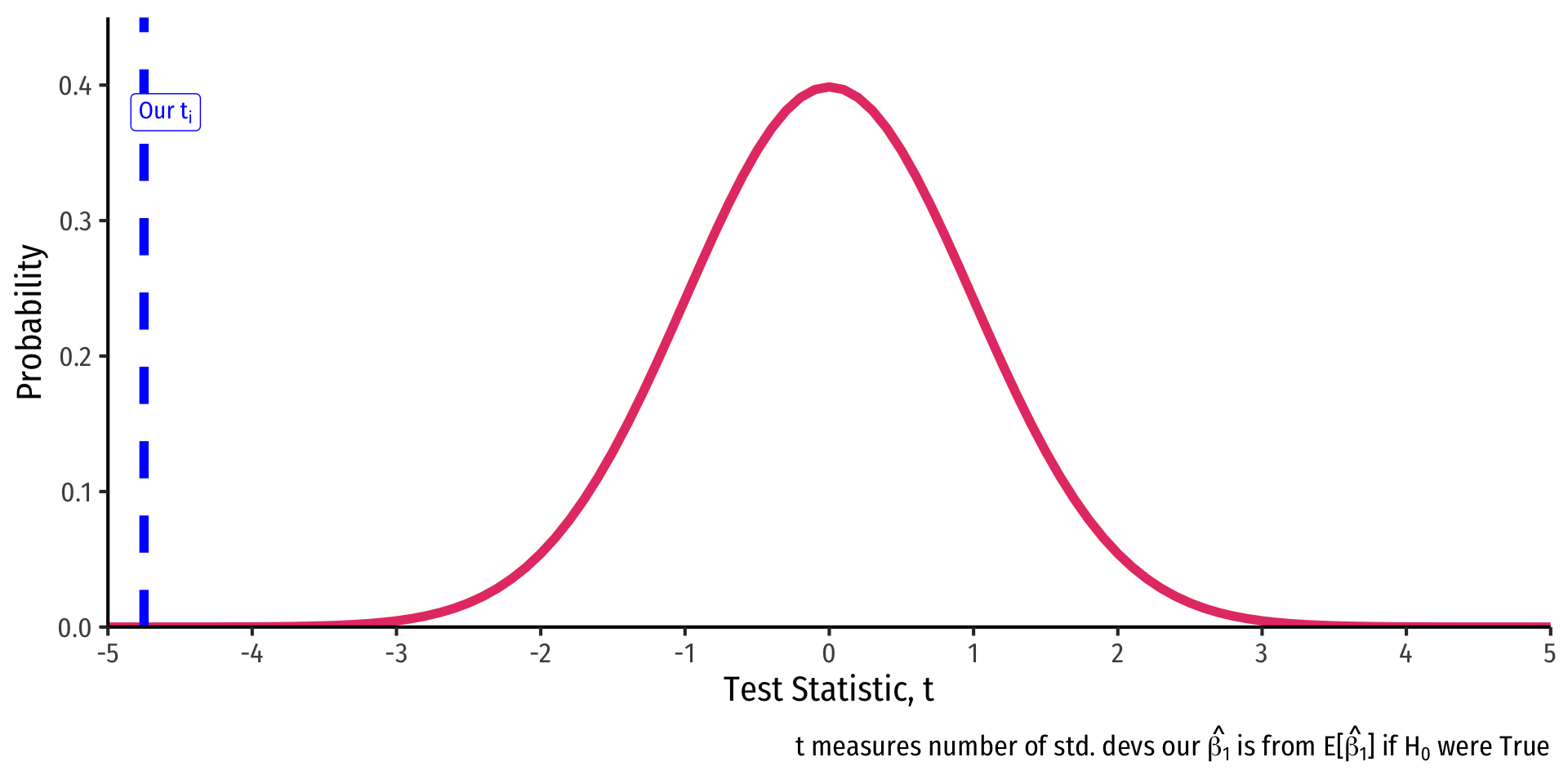
\(t\) same interpretation as \(Z\): number of std. dev. away from the sampling distribution’s expected value \(E[\hat{\beta_1}]\)1 (if \(H_0\) were true)
Compares to a critical value of \(t^*\) (pre-determined by \(\alpha\)-level & \(n-k-1\) df)
- For 95% confidence, \(\alpha=0.05\), \(t^* \approx 2\)2
What R Does: Theory-Based Statistical Inference III
\[\begin{align*} t &= \frac{\hat{\beta_1}-\beta_{1,0}}{se(\hat{\beta_1})}\\ t &= \frac{-2.28-0}{0.48}\\ t &= -4.75\\ \end{align*}\]
- Our sample slope \(\hat{\beta_1}\) is 4.75 standard deviations below the expected value \(E[\hat{\beta_1}]\) (i.e. 0) if \(H_0\) were true
What R Does: Theory-Based Statistical Inference IV
$$\[\begin{align*} t &= \frac{\hat{\beta_1}-\beta_{1,0}}{se(\hat{\beta_1})}\\ t &= \frac{-2.28-0}{0.48}\\ t &= -4.75\\ \end{align*}\]$$
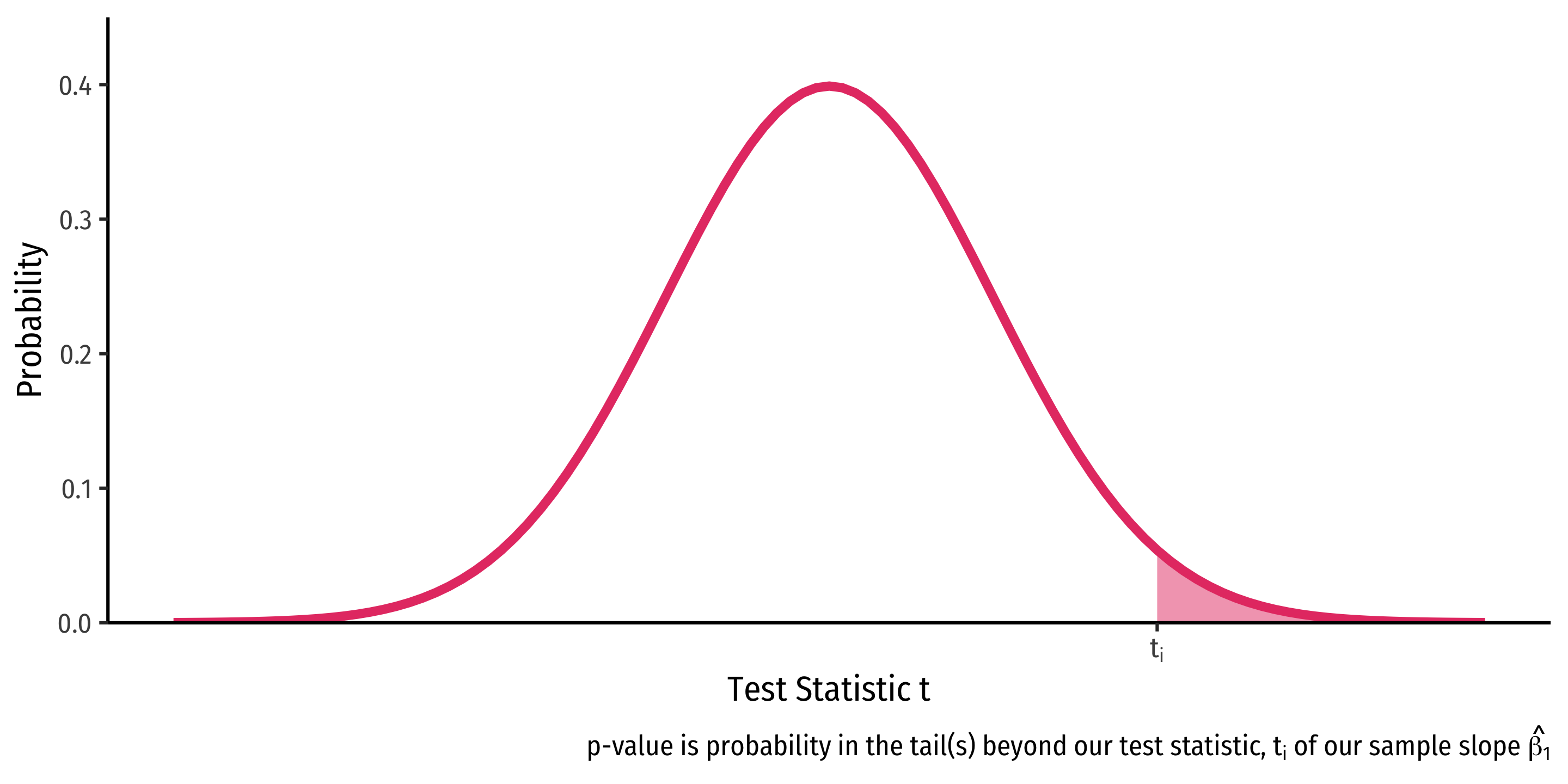
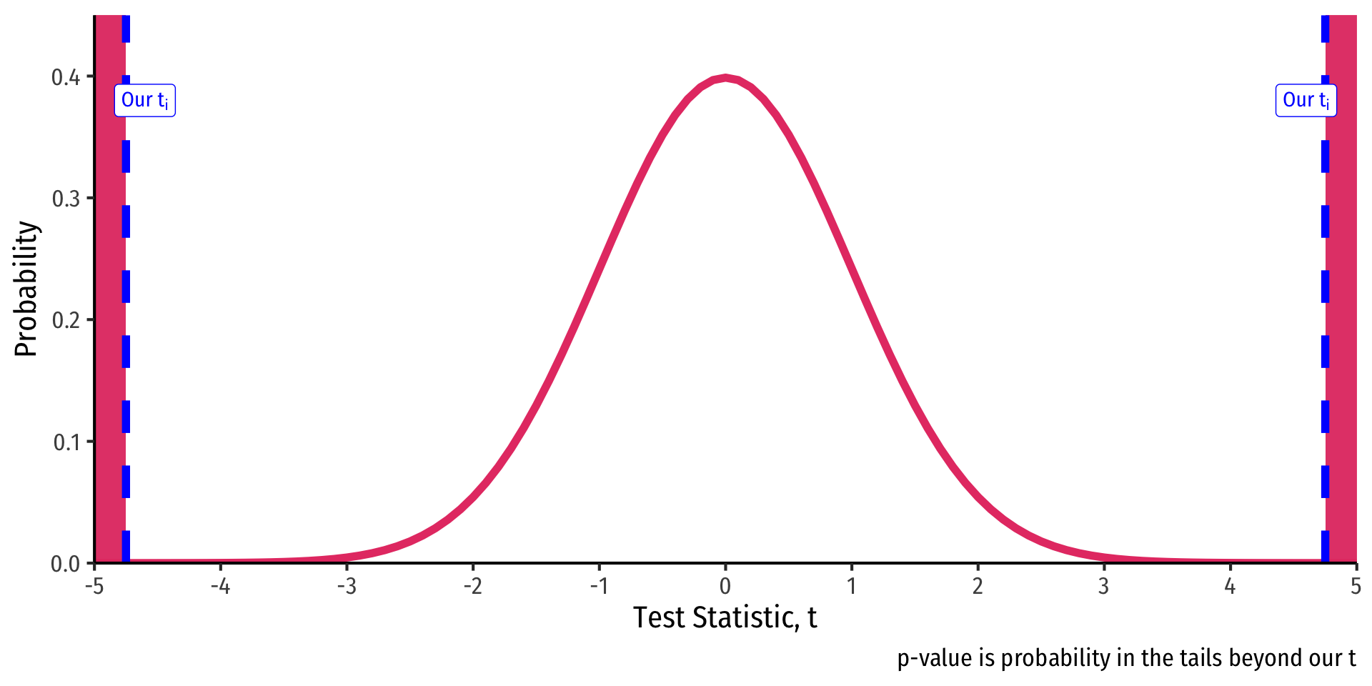
- .hi[p-value]: prob. of a test statistic at least as large (in magnitude) as ours if the null hypothesis were true
- Continuous distribution implies we need probability of area beyond our value
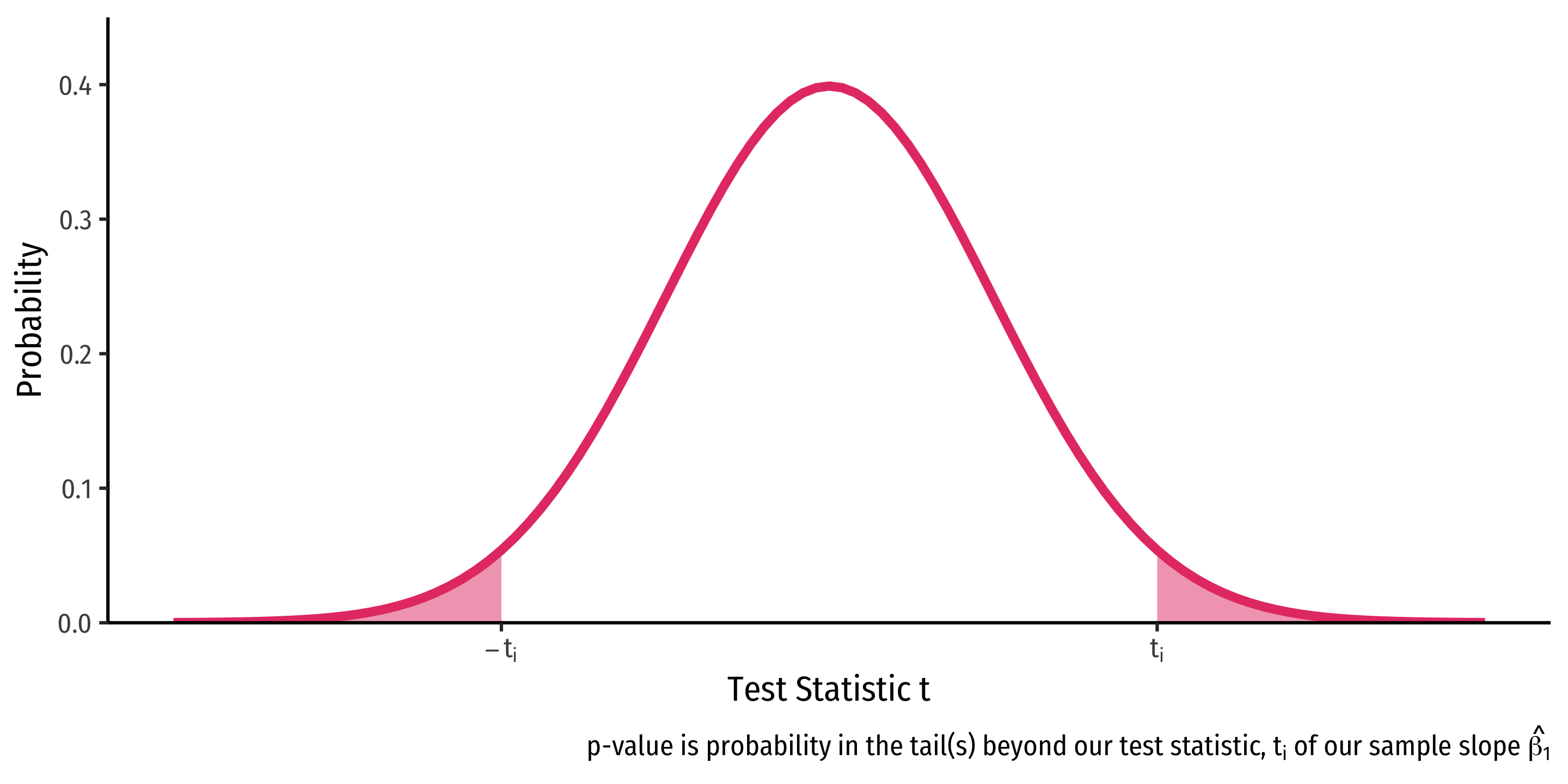
- p-value is 2-sided for \(H_a: \beta_1 \neq 0\)
- \(2 \times p(t_{418}> \vert -4.75\vert)=0.0000028\)

One-Sided Tests & p-Values
\(H_a: \beta_1<0\)
p-value: \(p(t \leq t_i)\)

\(H_a: \beta_1>0\)
p-value: \(p(t \geq t_i)\)
Two-Sided Tests and p-Values
\(H_a: \beta_1 \neq 0\)
p-value: \(2 \times p(t \geq |t_i|)\)
Calculating p-Values in R
pt()calculatesprobabilities on atdistribution with arguments:- the t-score
df =the degrees of freedomlower.tail =TRUEif looking at area to LEFT of valueFALSEif looking at area to RIGHT of value
- \(2 \times p(t_{418}> \vert -4.75\vert)=0.0000028\)
p-Hacking
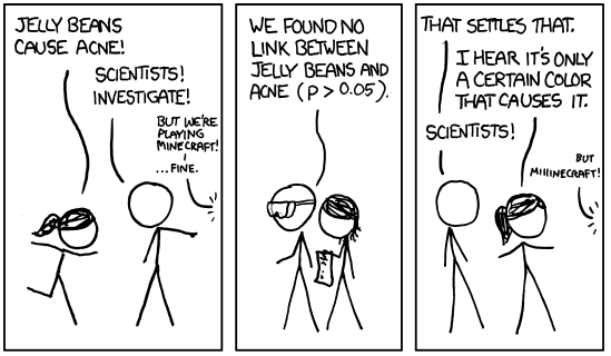
p-Hacking
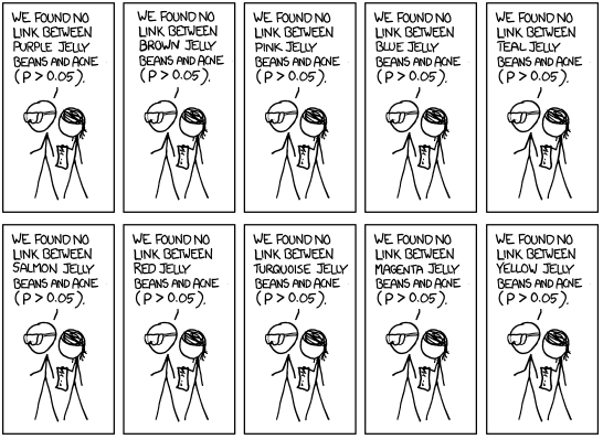
p-Hacking
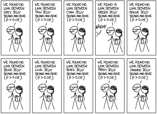
p-Hacking
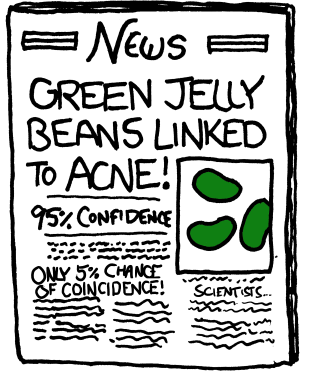
p-Hacking
Consider what 95% confident or \(\alpha=0.05\) means
If we repeat a procedure 20 times, we should expect \(\frac{1}{20}\) (5%) to produce a fluke result!
Image source: Seeing Theory
Abusing p-values and “Science”
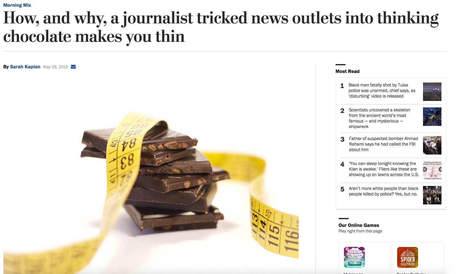
Source: Washington Post
Abusing p-Values and “Science” I
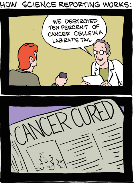

Source: SMBC
Abusing p-Values and “Science” II

“The widespread use of ‘statistical significance’ (generally interpreted as \((p \leq 0.05)\) as a license for making a claim of a scientific finding (or implied truth) leads to considerable distortion of the scientific process.”
Wasserstein, Ronald L. and Nicole A. Lazar, (2016), “The ASA’s Statement on p-Values: Context, Process, and Purpose,” The American Statistician 30(2): 129-133
Abusing p-Values and “Science” III
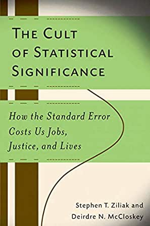
“No economist has achieved scientific success as a result of a statistically significant coefficient. Massed observations, clever common sense, elegant theorems, new policies, sagacious economic reasoning, historical perspective, relevant accounting, these have all led to scientific success. Statistical significance has not,” (p.112).
McCloskey, Dierdre N and Stephen Ziliak, 1996, The Cult of Statistical Significance
Statistical Significance In Regression Tables
| Test Score | |
|---|---|
| Constant | 698.93*** |
| (9.47) | |
| STR | −2.28*** |
| (0.48) | |
| n | 420 |
| R2 | 0.05 |
| SER | 18.54 |
| * p < 0.1, ** p < 0.05, *** p < 0.01 |
- Statistical significance is shown by asterisks, common (but not always!) standard:
- 1 asterisk: significant at \(\alpha=0.10\)
- 2 asterisks: significant at \(\alpha=0.05\)
- 3 asterisks: significant at \(\alpha=0.01\)
- Rare, but sometimes regression tables include \(p\)-values for estimates
