You Don’t Need an RCT to Talk About Causality
Statistics profession is obstinant that we cannot say anything about causality
But you have to! It’s how the human brain works!
We can’t conceive of (spurious) correlation without some causation

The Causal Revolution

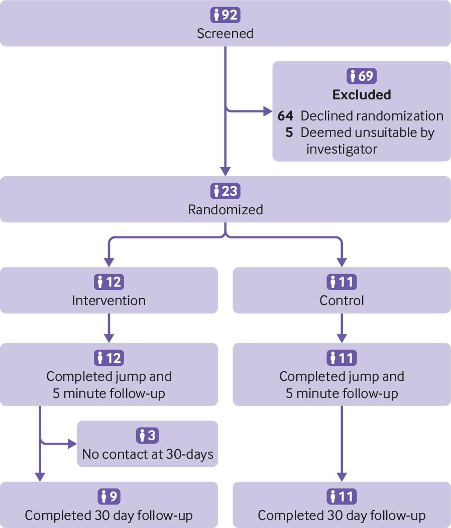
RCTs and Evidence-Based Policy
Should we ONLY base policies on the evidence from Randomized Controlled Trials
| ̄ ̄ ̄ ̄ ̄ ̄ ̄ ̄ ̄ ̄|
— Ellie Murray (@EpiEllie) July 13, 2018
IF U DONT SMOKE,
U ALREADY
BELIEVE IN
CAUSAL INFERENCE
WITHOUT
RANDOMIZED TRIALS
|__________|
(__/) ||
(•ㅅ•) ||
/ づ#HistorianSignBunny #Epidemiology
Source: British Medical Journal

RCTs and Evidence-Based Policy II
RCTs and Evidence-Based Policy II

What Does Causation Mean?
- “Correlation does not imply causation”
- this is exactly backwards!
- this is just pointing out that exogeneity is violated
What Does Causation Mean?
- “Correlation does not imply causation”
- this is exactly backwards!
- this is just pointing out that exogeneity is violated
- “Correlation implies causation”
- for an association, there must be some causal chain that relates \(X\) and \(Y\)
- but not necessarily merely \(X \rightarrow Y\)
- “Correlation plus exogeneity is causation.”
Correlation and Causation
- Correlation:
- Math & Statistics
- Computers, AI, Machine learning can figure this out (better than humans)
- Causation:
- Philosophy, Intuition, Theory
- Counterfactual thinking, unique to humans (vs. animals or computers)
- Computers cannot (yet) figure this out
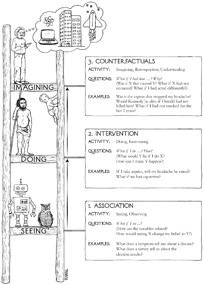
The Causal Revolution


Causation Requires Counterfactual Thinking

Causal Inference
We will seek to understand what causality is and how we can approach finding it
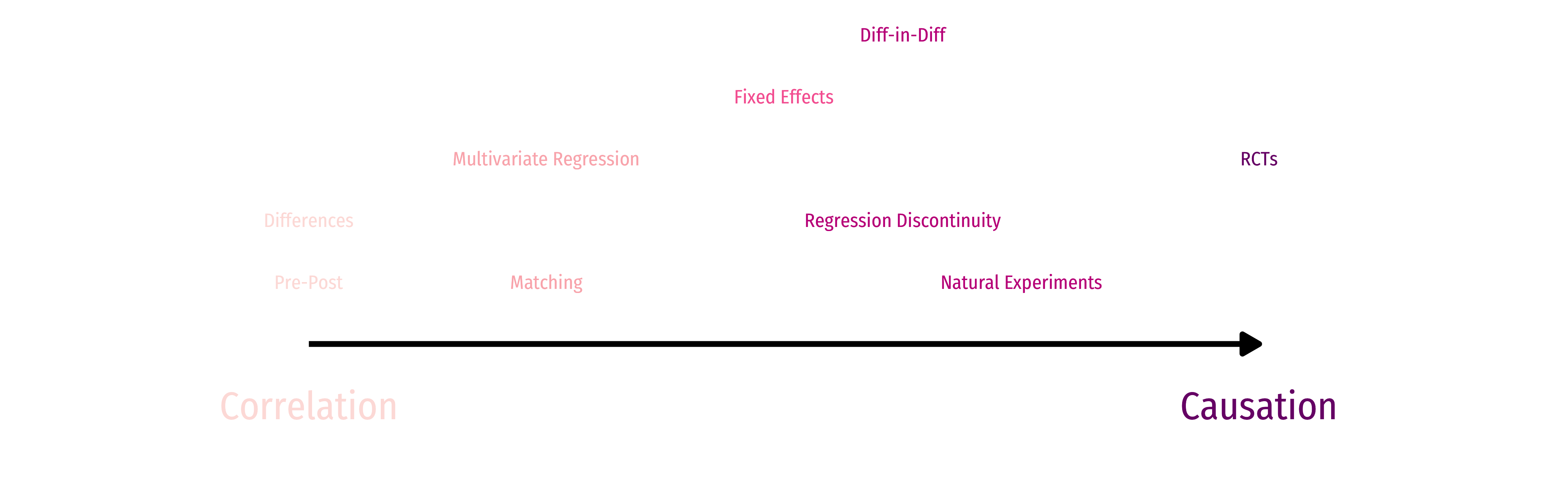
We will also explore the different common research designs meant to identify causal relationships
These skills, more than supply & demand, constrained optimization models, ISLM, etc, are the tools and comparative advantage of a modern research economist
- Why all big companies (especially in tech) have entire economics departments in them

Clever Research Designs Identify Causality
What Then IS Causation?
- \(X\) causes \(Y\) if we can intervene and change \(X\) without changing anything else, and \(Y\) changes
- \(Y\) “listens to” \(X\)
- \(X\) may not be the only thing that causes \(Y\)!

What Then IS Causation?
- \(X\) causes \(Y\) if we can intervene and change \(X\) without changing anything else, and \(Y\) changes
- \(Y\) “listens to” \(X\)
- \(X\) may not be the only thing that causes \(Y\)!
Counterfactuals
The sine qua non of causal claims are counterfactuals: what would \(Y\) have been if \(X\) had been different?
It is impossible to make a counterfactual claim from data alone!
Need a (theoretical) causal model of the data-generating process!
Counterfactuals and RCTs
Again, RCTs are invoked as the gold standard for their ability to make counterfactual claims:
Treatment/intervention \((X)\) is randomly assigned to individuals
If person i who recieved treatment had not recieved the treatment, we can predict what his outcome would have been
If person j who did not recieve treatment had recieved treatment, we can predict what her outcome would have been
- We can say this because, on average, treatment and control groups are the same before treatment
From RCTs to Causal Models
RCTs are but the best-known method of a large, growing science of causal inference
We need a causal model to describe the data-generating process (DGP)
Requires us to make some assumptions
Causal Diagrams/DAGs
A visual model of the data-generating process, encodes our understanding of the causal relationships
Requires some common sense/economic intuition
Remember, all models are wrong, we just need them to be useful!
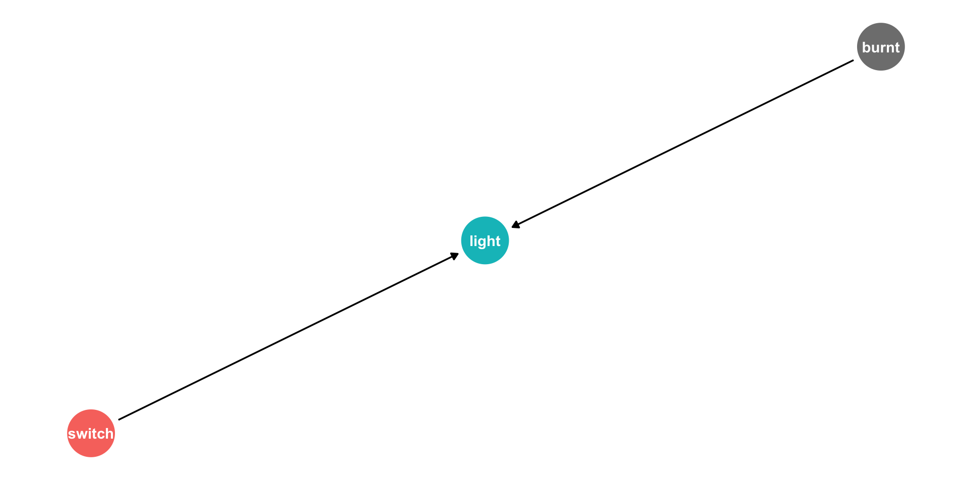
Causal Diagrams/DAGs
- Our light switch example of causality
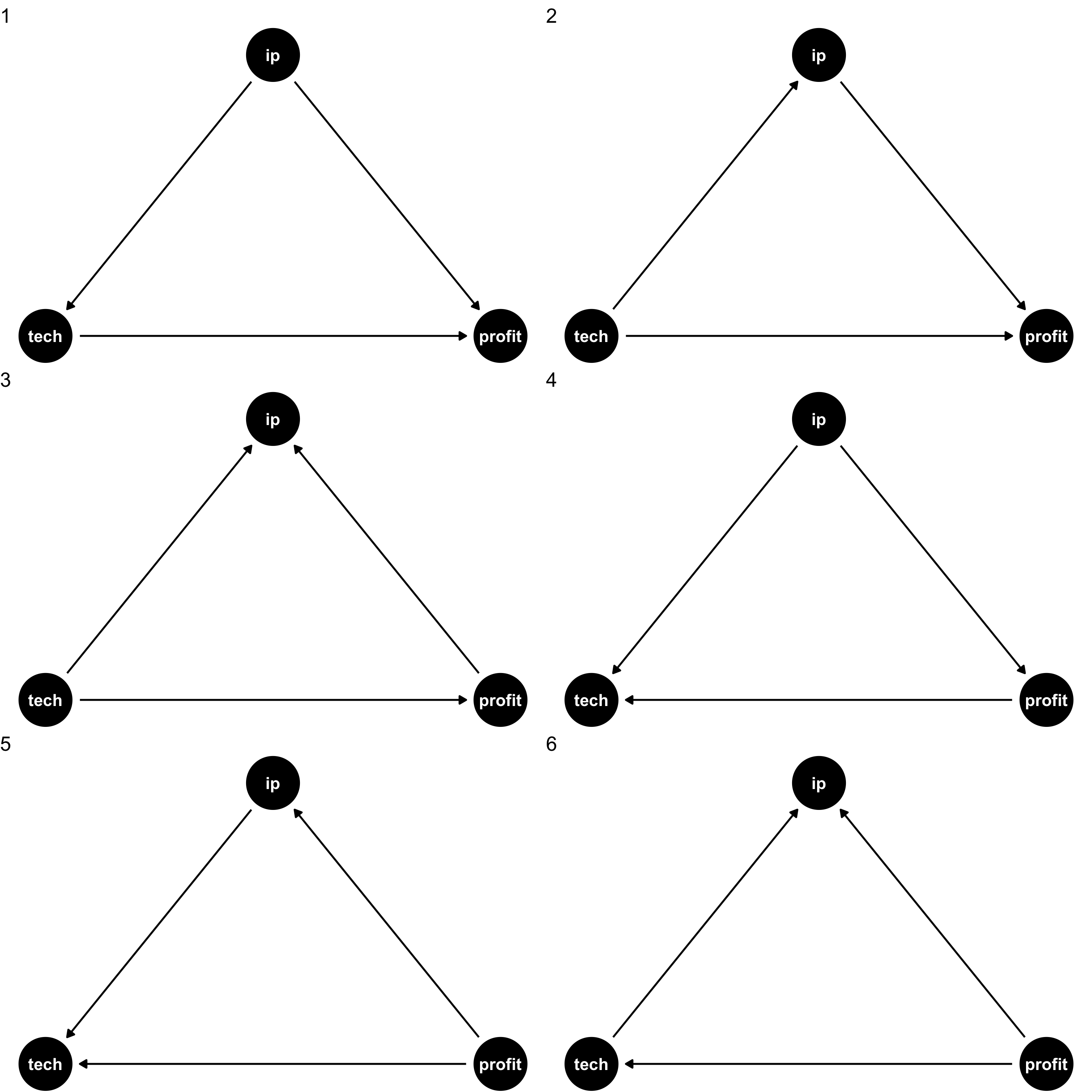
Drawing a DAG: Example
Suppose we have data on three variables
IP: how much a firm spends on IP lawsuitstech: whether a firm is in tech industryprofit: firm profits
They are all correlated with each other, but what’s are the causal relationships?
We need our own causal model (from theory, intuition, etc) to sort
- Data alone will not tell us!
Drawing a DAG
Consider all the variables likely to be important to the data-generating process (including variables we can’t observe!)
For simplicity, combine some similar ones together or prune those that aren’t very important
Consider which variables are likely to affect others, and draw arrows connecting them
Test some testable implications of the model (to see if we have a correct one!)

Drawing a DAG
Drawing an arrow requires a direction - making a statement about causality!
Omitting an arrow makes an equally important statement too!
- In fact, we will need omitted arrows to show causality!
If two variables are correlated, but neither causes the other, likely they are both caused by another (perhaps unobserved) variable - add it!
There should be no cycles or loops (if so, there’s probably another missing variable, such as time)
DAG Example I

DAG Example I
- What other variables are important?
- Ability
- Socioeconomic status
- Demographics
- Phys. Ed. requirements
- Year of birth
- Location
- Schooling laws
- Job connections

DAG Example I
In social science and complex systems, 1000s of variables could plausibly be in DAG!
So simplify:
- Ignore trivial things (Phys. Ed. requirement)
- Combine similar variables (Socioeconomic status, Demographics, Location) \(\rightarrow\) Background
DAG Example II
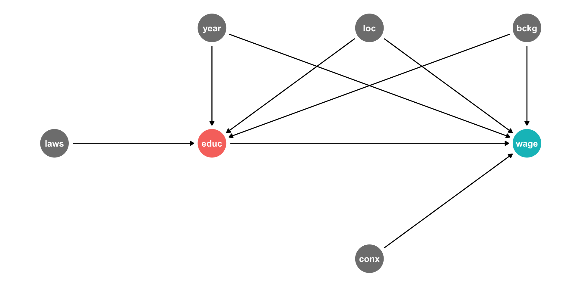
Background, Year of birth, Location, Compulsory schooling, all cause education
Background, year of birth, location, job connections probably cause wages
DAG Example II
Background, Year of birth, Location, Compulsory schooling, all cause education
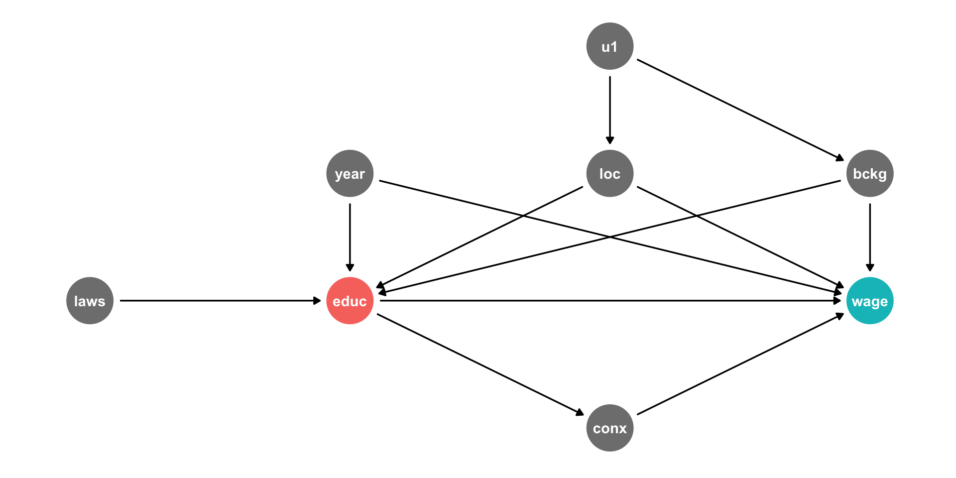
Background, year of birth, location, job connections probably cause wages
Job connections in fact is probably caused by education!
Location and background probably both caused by unobserved factor (
u1)
DAG Example II
This is messy, but we have a causal model!
Makes our assumptions explicit, and many of them are testable
DAG suggests certain relationships that will not exist:
- all relationships between
lawsandconxgo througheduc - so if we controlled for
educ, thencor(laws,conx)should be zero!
- all relationships between

Let the Computer Do It: Dagitty.net I

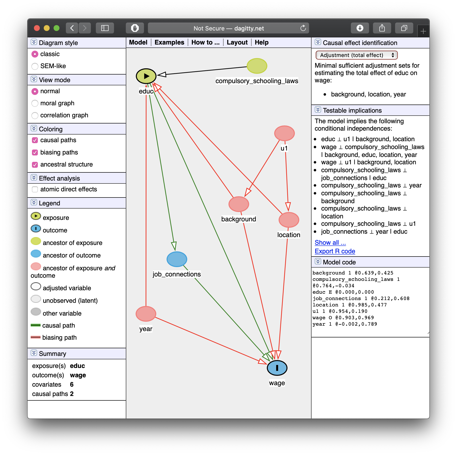
Dagitty.net is a great tool to make these and give you testable implications
Click
Model -> New ModelName your “exposure” variable \((X\) of interest) and “outcome” variable \((Y)\)
Let the Computer Do It: Dagitty.net II

Click and drag to move nodes around
Add a new variable by double-clicking
Add an arrow by double-clicking one variable and then double-clicking on the target (do again to remove arrow)
Let the Computer Do It: Dagitty.net II
Let the Computer Do It: Dagitty.net III
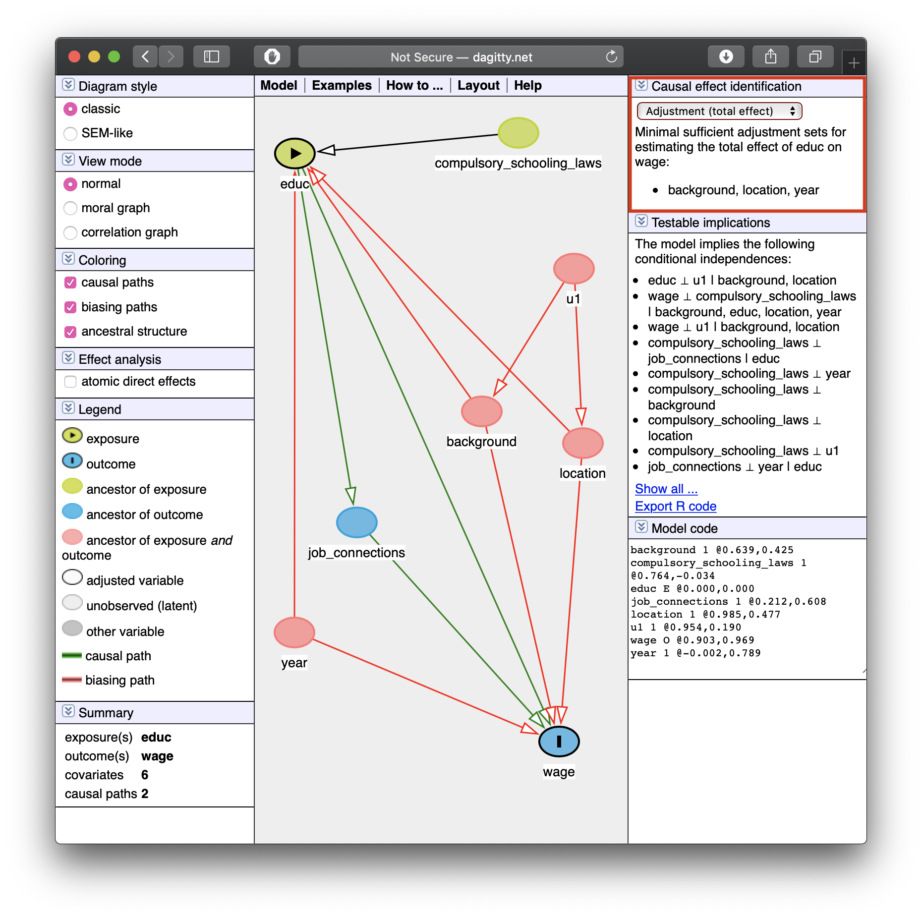
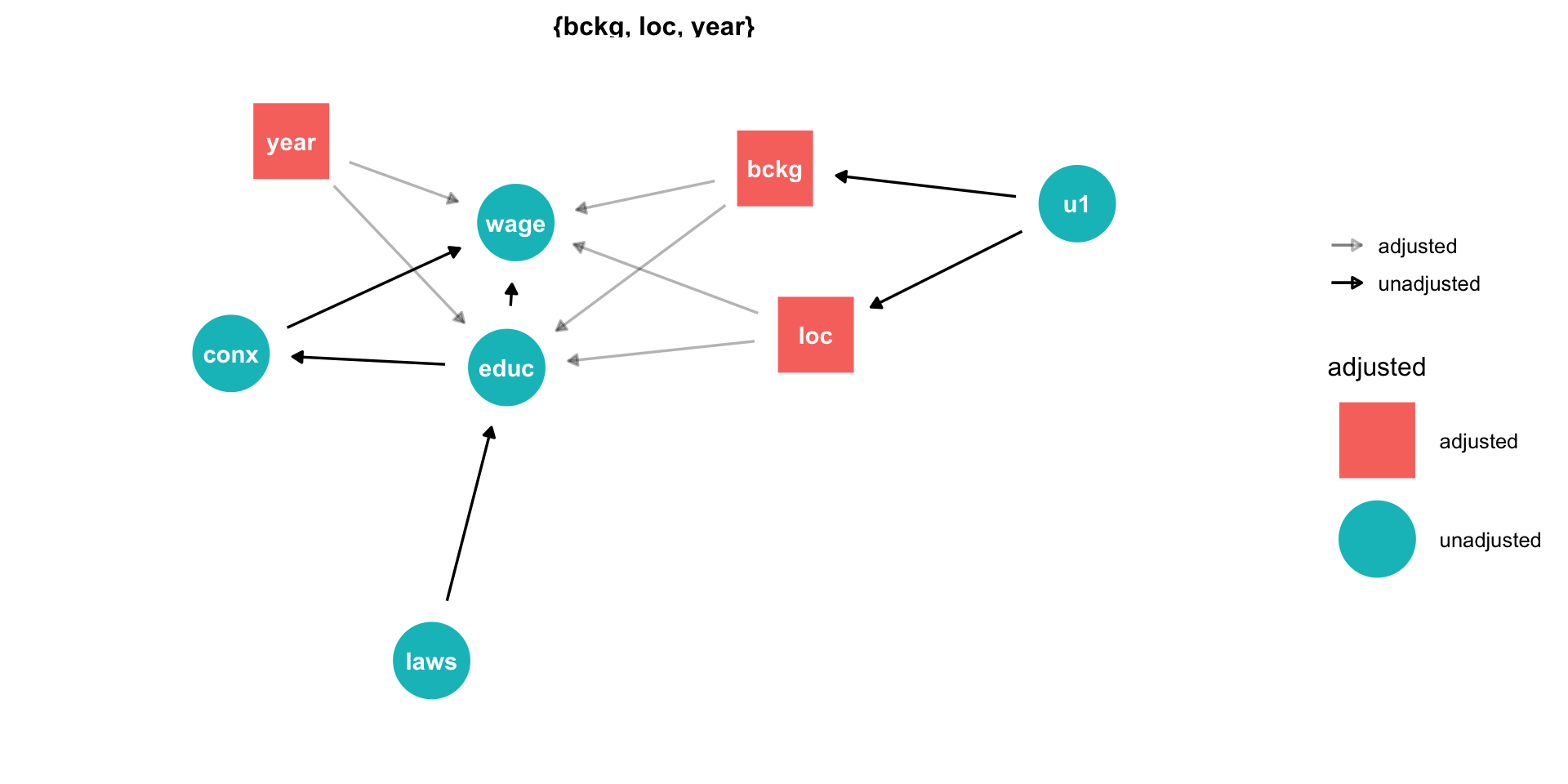
- Tells you how to identify your effect! (upper right)
Minimal sufficient adjustment sets containing background, location, year for estimating the total effect of educ on wage: background, location, year
Let the Computer Do It: Dagitty.net III
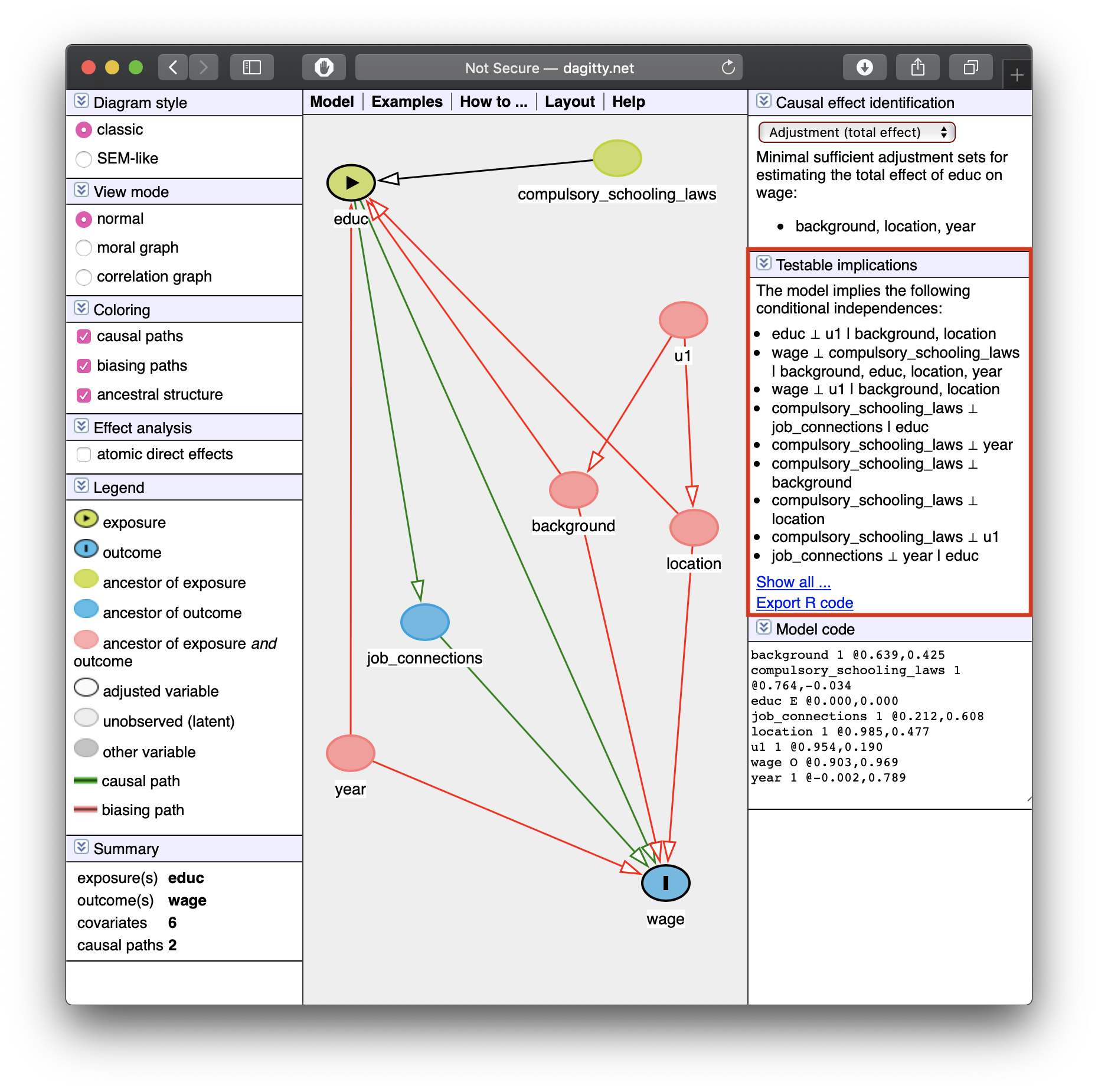
Tells you some testable implications of your model
These are (conditional) independencies:
\[X \perp Y \, | \, Z\]
“X is independent of Y, given Z”
- Implies that by controlling for \(Z\), \(X\) and \(Y\) should have no correlation
Let the Computer Do It: Dagitty.net III
Tells you some testable implications of your model
Example: look at the last one listed:
job_connections \(\perp\) year \(\vert\) educ
“Job connections are independent of year, controlling for education”
- Implies that by controlling for
educ, there should be no correlation betweenjob_connectionsandyear— can test this with data!
Causal Effect
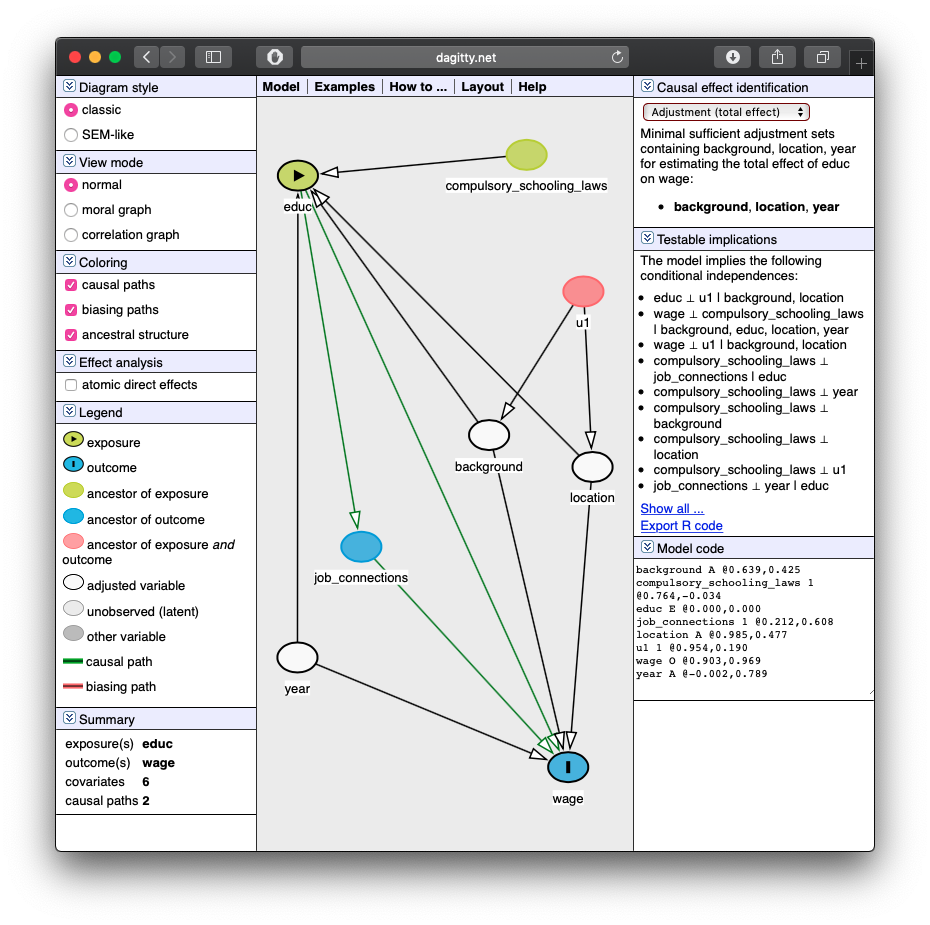
- If we control for
background,location, andyear, we can identify the causal effect ofeduc\(\rightarrow\)wage.
You Can Draw DAGs in R
- New package:
ggdag - Arrows are made with formula notation:
Y ~ X + Zmeans “Yis caused byXandZ”
You Can Draw DAGs in R II
- Or you can just copy the code from
dagitty.net! - Use
dagitty()from thedagittypackage, and paste the code in quotes
# install.packages("dagitty")
library(dagitty)
dagitty('dag {
bb="0,0,1,1"
background [pos="0.413,0.335"]
compulsory_schooling_laws [pos="0.544,0.076"]
educ [exposure,pos="0.185,0.121"]
job_connections [pos="0.302,0.510"]
location [pos="0.571,0.431"]
u1 [pos="0.539,0.206"]
wage [outcome,pos="0.552,0.761"]
year [pos="0.197,0.697"]
background -> educ
background -> wage
compulsory_schooling_laws -> educ
educ -> job_connections
educ -> wage
job_connections -> wage
location -> educ
location -> wage
u1 -> background
u1 -> location
year -> educ
year -> wage
}') %>%
  ggdag()+
  theme_dag()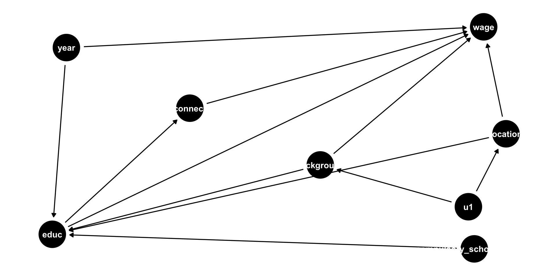
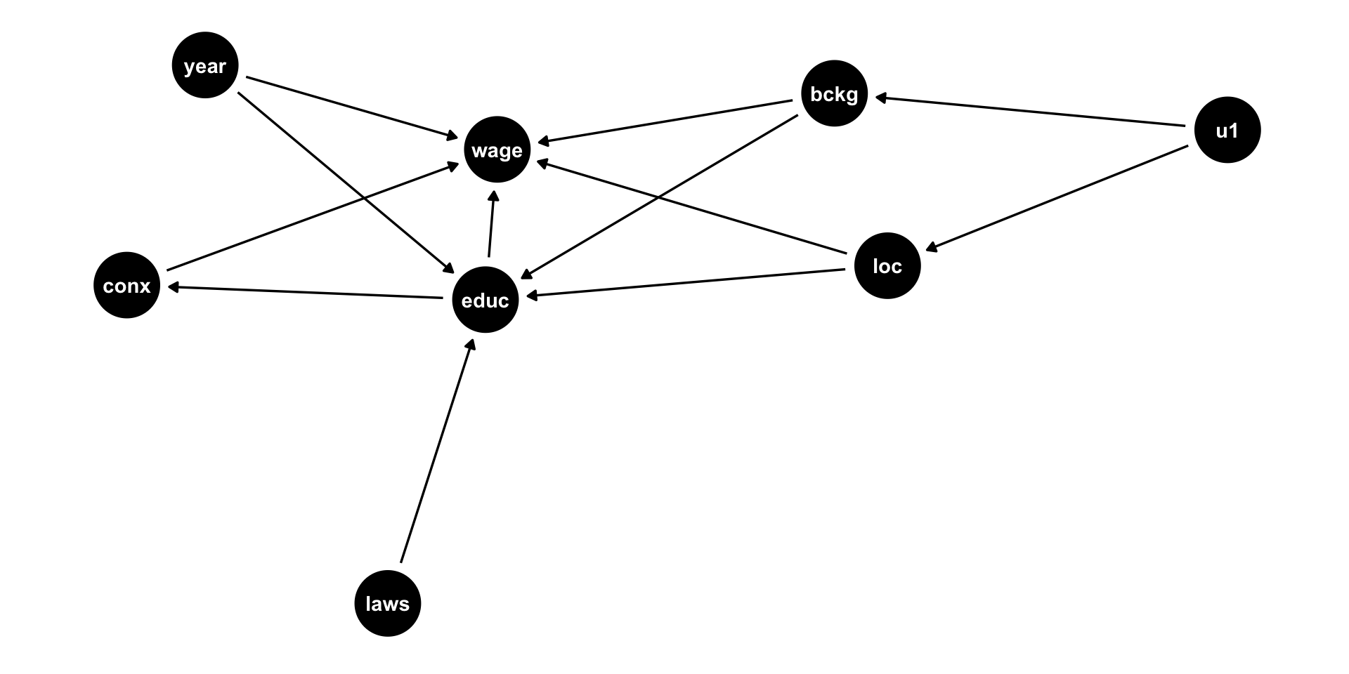
You Can Draw DAGs In R
- It’s not very pretty, but if you set
text = FALSE, use_labels = "nameinsideggdag(), makes it easier to read
dagitty('dag {
bb="0,0,1,1"
background [pos="0.413,0.335"]
compulsory_schooling_laws [pos="0.544,0.076"]
educ [exposure,pos="0.185,0.121"]
job_connections [pos="0.302,0.510"]
location [pos="0.571,0.431"]
u1 [pos="0.539,0.206"]
wage [outcome,pos="0.552,0.761"]
year [pos="0.197,0.697"]
background -> educ
background -> wage
compulsory_schooling_laws -> educ
educ -> job_connections
educ -> wage
job_connections -> wage
location -> educ
location -> wage
u1 -> background
u1 -> location
year -> educ
year -> wage
}') %>%
  ggdag(., text = FALSE, use_labels = "name")+
  theme_dag()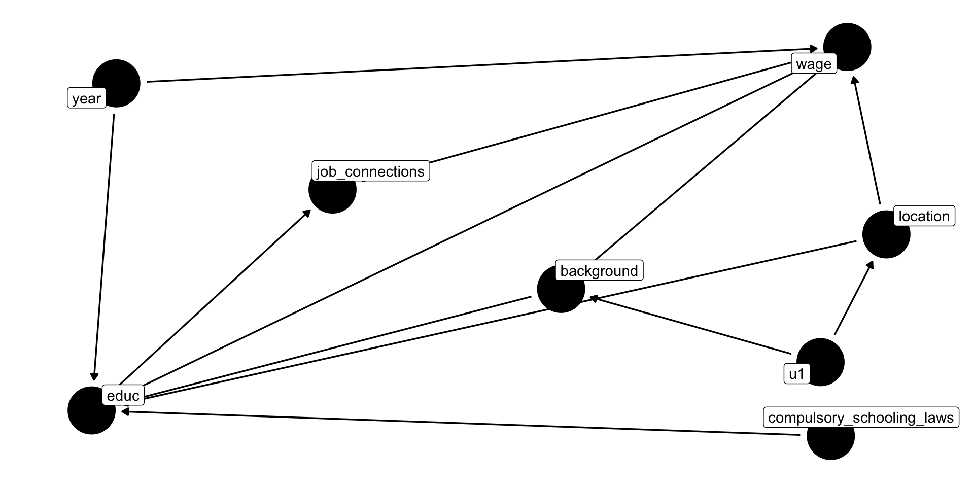
ggdag: Additional Tools
- If you have defined
X(exposure) andY(outcome), you can useggdag_paths()to have it show all possible paths between \(X\) and \(Y\)!
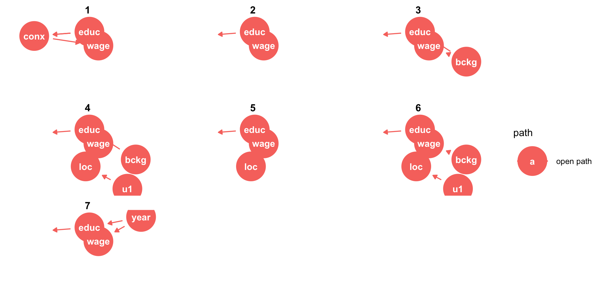
ggdag: Additional Tools
- If you have defined
X(exposure) andY(outcome), you can useggdag_adjustment_set()to have it show you what you need to control for in order to identify \(X \rightarrow Y\)!
DAG Rules
How does dagitty.net and
ggdagknow how to identify effects, or what to control for, or what implications are testable?Comes from fancy math called “do-calculus”
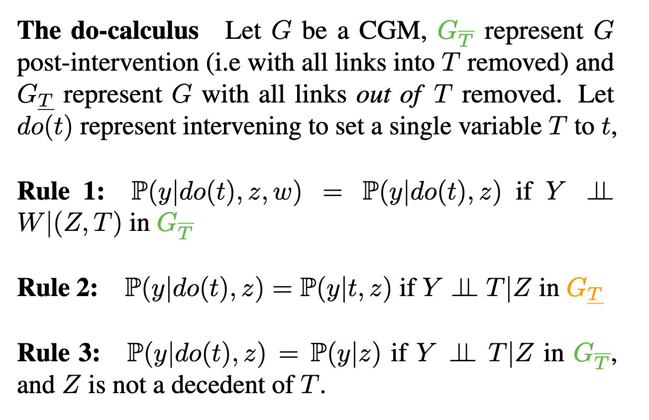
- Fortunately, these amount to a few simple rules that we can see on a DAG
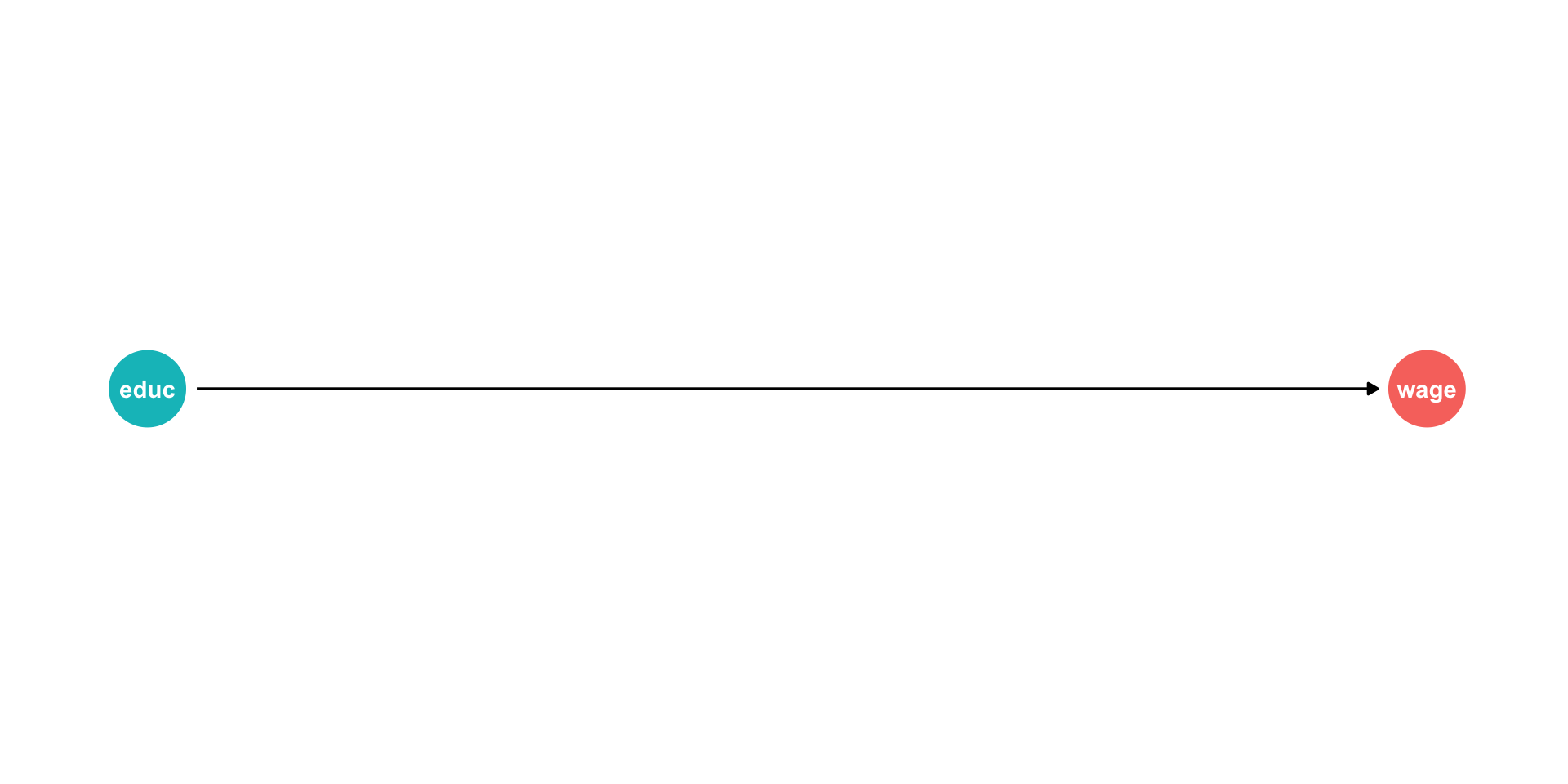
DAGs I
Typical notation:
\(X\) is independent variable of interest
- Epidemiology: “intervention” or “exposure”
\(Y\) is dependent or “response” variable
Other variables use other letters
You can of course use words instead of letters!
DAGs and Causal Effects
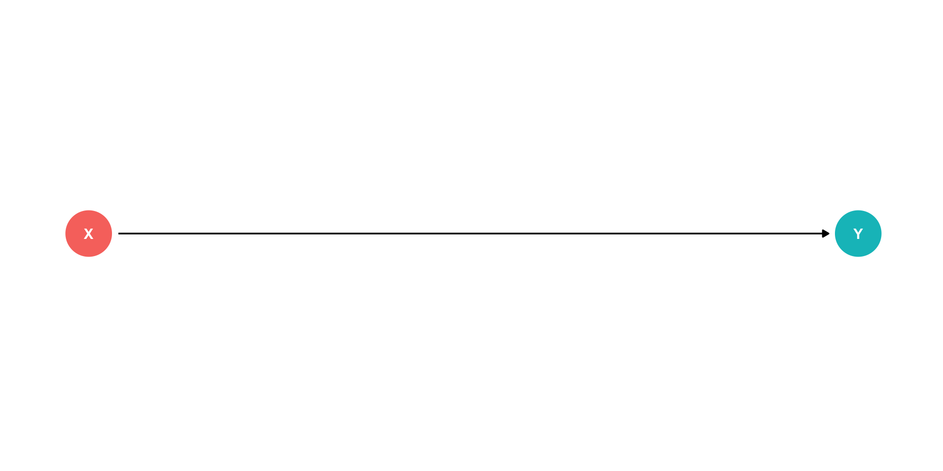
Arrows indicate causal effect (& direction)
Two types of causal effect:
- Direct effects: \(X \rightarrow Y\)

DAGs and Causal Effects
Arrows indicate causal effect (& direction)
Two types of causal effect:
Direct effects: \(X \rightarrow Y\)
Indirect effects: \(X \rightarrow M \rightarrow Y\)
- \(M\) is a “mediator” variable, the mechanism by which \(X\) affects \(Y\)
DAGs and Causal Effects
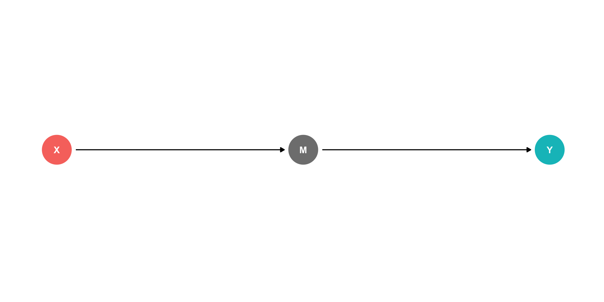
Arrows indicate causal effect (& direction)
Two types of causal effect:
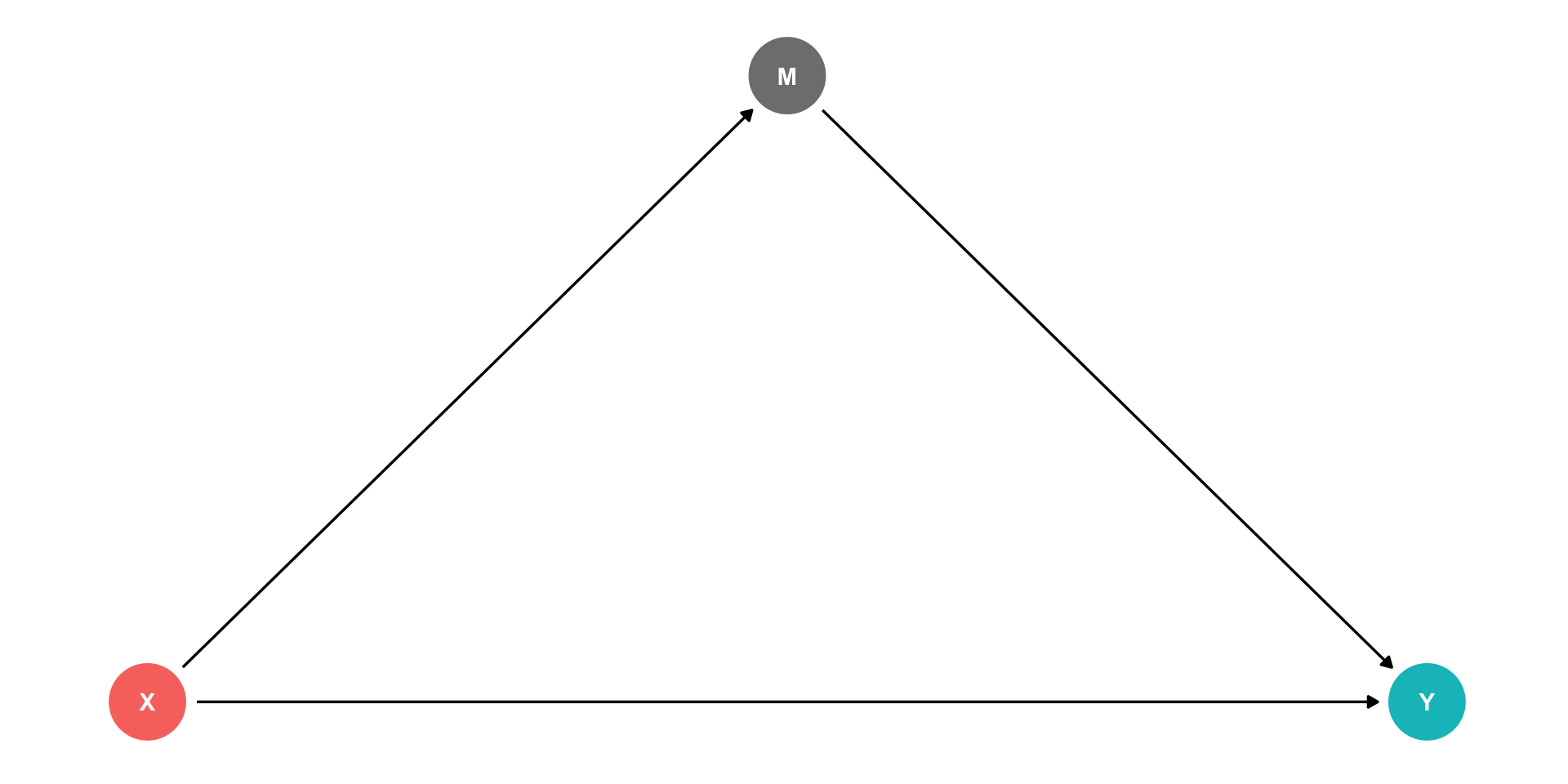
Direct effects: \(X \rightarrow Y\)
Indirect effects: \(X \rightarrow M \rightarrow Y\)
- \(M\) is a “mediator” variable, the mechanism by which \(X\) affects \(Y\)
- You of course might have both!
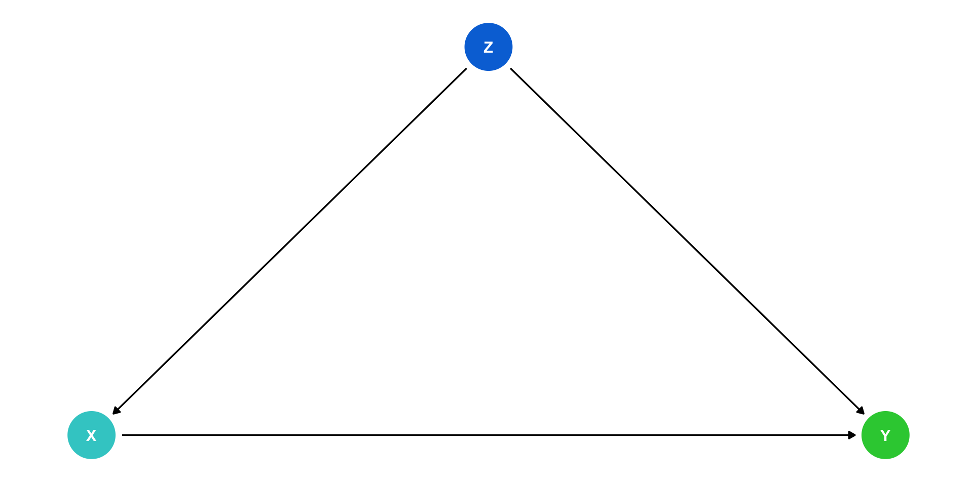
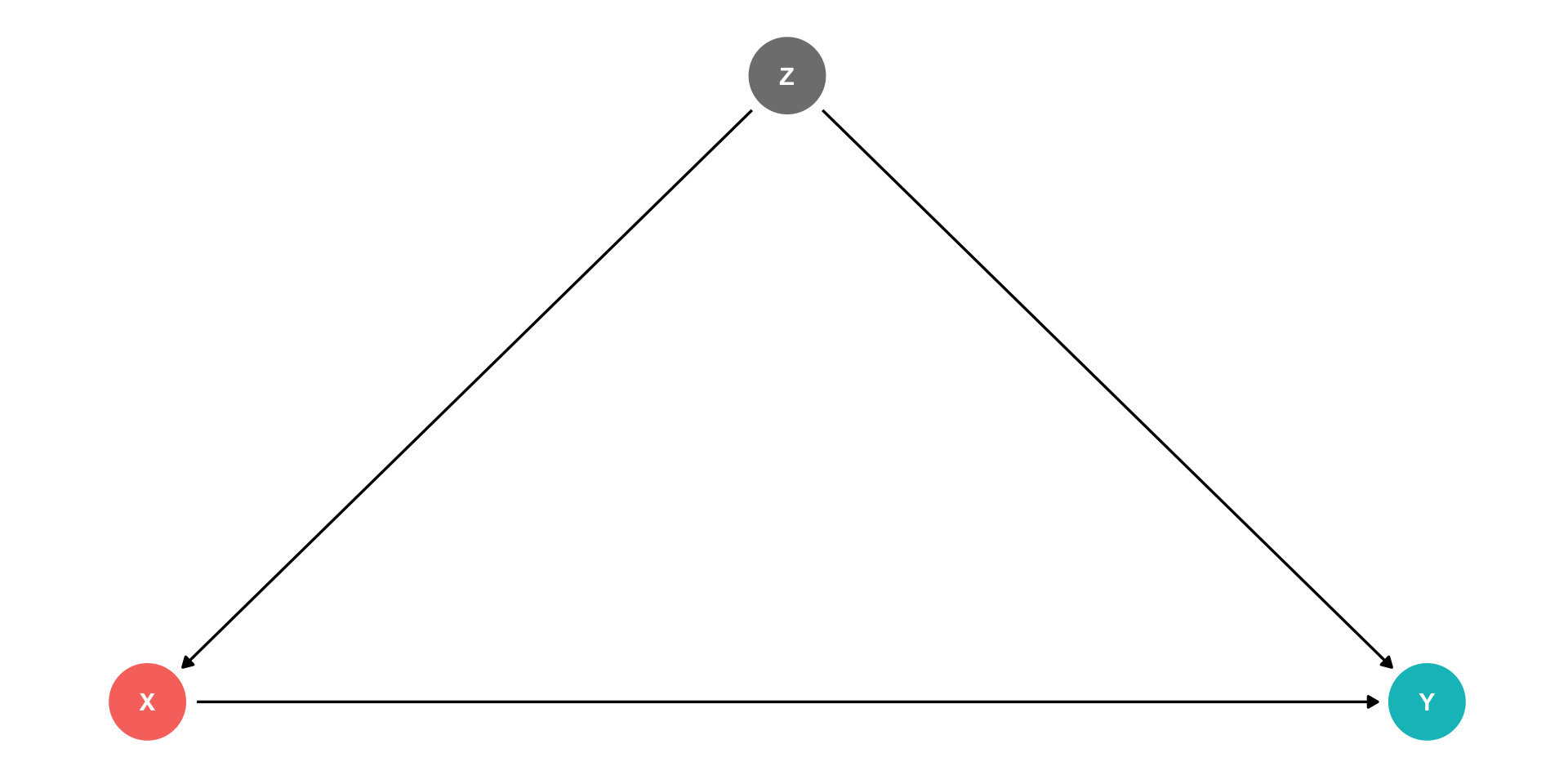
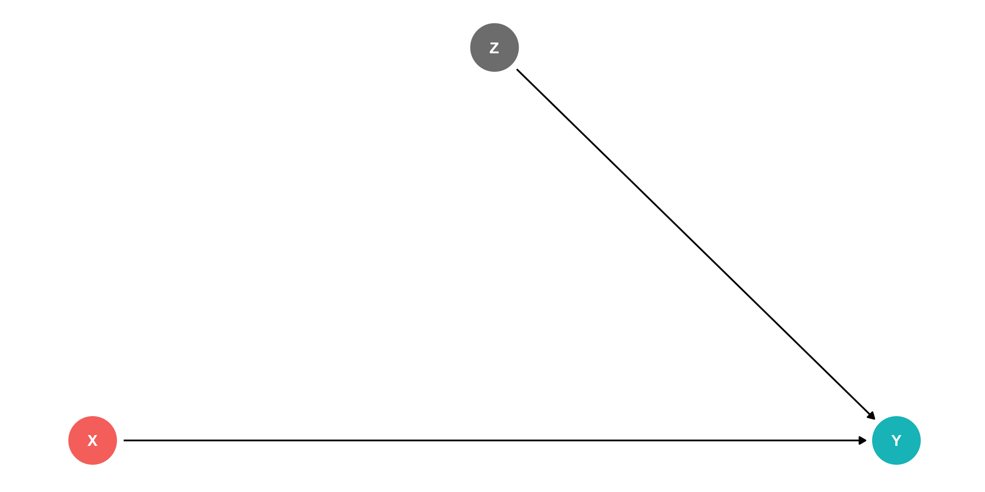
Confounders
\(Z\) is a “confounder”: it causes both \(X\) and \(Y\)
\(cor(X,Y)\) is made up of two parts:
- Causal effect of \((X \rightarrow Y)\) 👍
- \(Z\) causing both the values of \(X\) and \(Y\) 👎
Failing to control for \(Z\) will bias our estimate of the causal effect of \(X \rightarrow Y\)!

Confounders
- Confounders are the DAG-equivalent of omitted variable bias (next class)
\[Y_i=\beta_0+\beta_1 X_i\]
By leaving out \(Z_i\), this regression is biased
\(\hat{\beta}_1\) picks up both:
- \(X \rightarrow Y\)
- \(X \leftarrow Z \rightarrow Y\)
“Front Doors” and “Back Doors”
- With this DAG, there are 2 paths that connect \(X\) and \(Y\)1:
- A causal “front-door” path: \(X \rightarrow Y\)
- 👍 what we want to measure
- A non-causal “back-door” path: \(X \leftarrow Z \rightarrow Y\)
- At least one causal arrow runs in the opposite direction
- 👎 adds a confounding bias

Controlling I
Ideally, if we ran a randomized control trial and randomly assigned different values of \(X\) to different individuals, this would delete the arrow between \(Z\) and \(X\)
- Individuals’ values of \(Z\) do not affect whether or not they are treated (\(X\))
This would only leave the front-door, \(X \rightarrow Y\)
But we can rarely run an ideal RCT
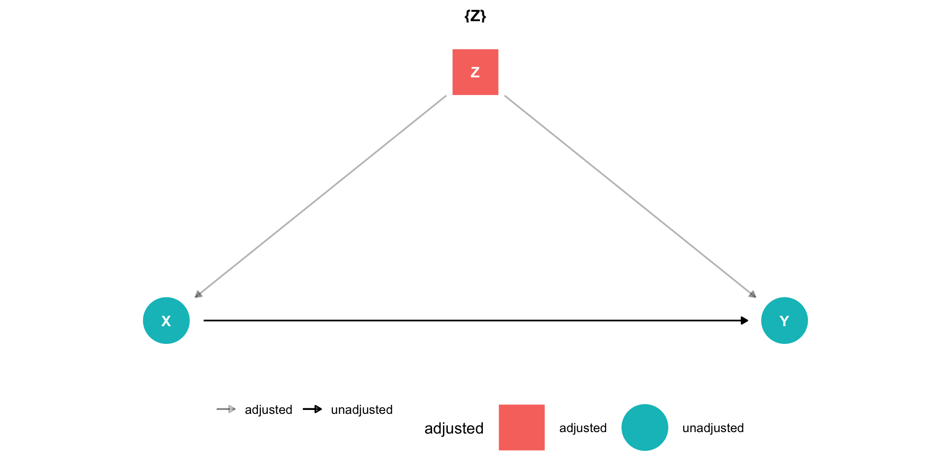
Controlling II
Instead of an RCT, if we can just “adjust for” or “control for” \(Z\), we can block the back-door path \(X \leftarrow Z \rightarrow Y\)
This would only leave the front-door path open, \(X \rightarrow Y\)
“As good as” an RCT!
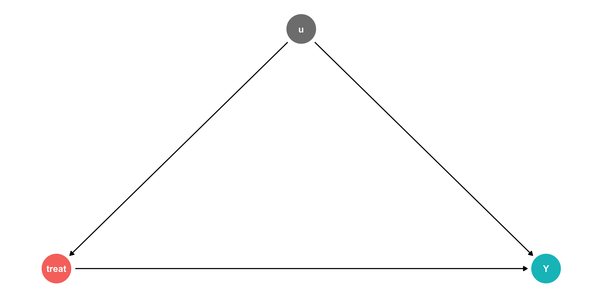
Controlling II
Using our terminology from last class, we have an outcome \((Y)\), and some treatment
But there are unobserved factors \((u)\)
\[Y_i = \beta_0 + \beta_1 Treatment + u_i\]
Controlling II
Using our terminology from last class, we have an outcome \((Y)\), and some treatment
But there are unobserved factors \((u)\)
\[Y_i = \beta_0 + \beta_1 Treatment + u_i\]
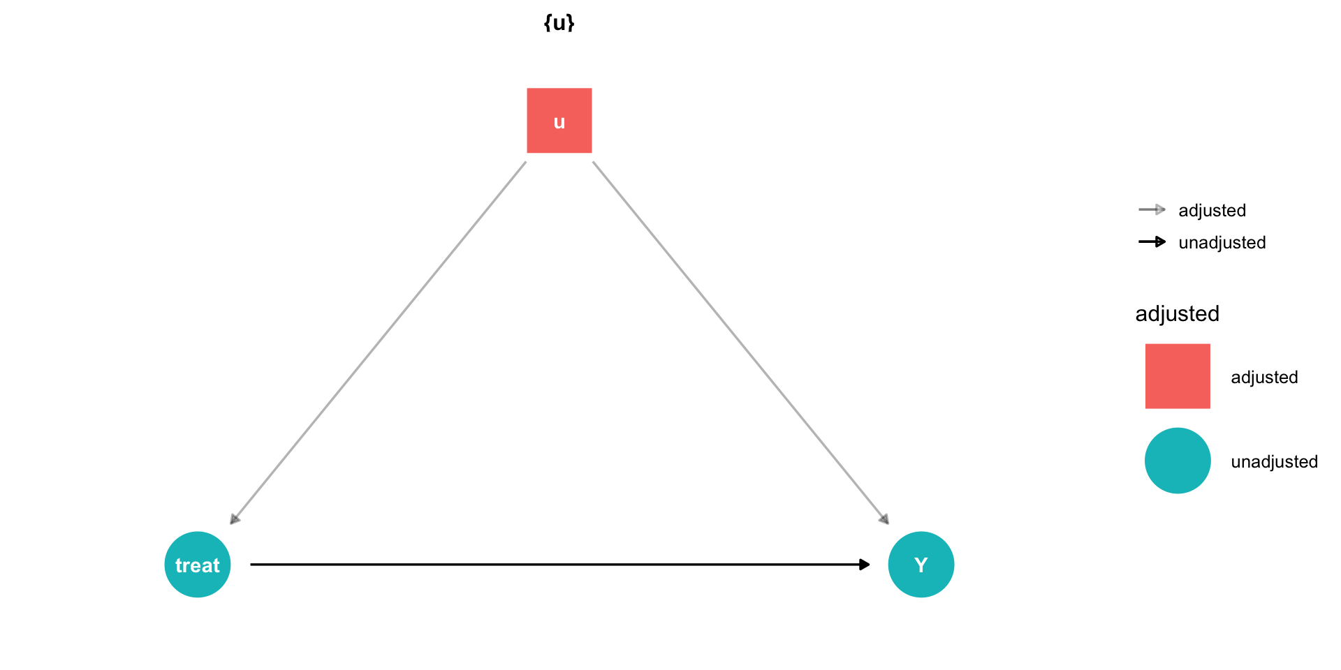
- If we can randomly assign treatment, this makes treatment exogenous:
\[cor(treatment,u)=0\]

Controlling II
Using our terminology from last class, we have an outcome \((Y)\), and some treatment
But there are unobserved factors \((u)\)
\[Y_i = \beta_0 + \beta_1 Treatment + u_i\]
- When we (often) can’t randomly assign treatment, we have to find another way to control for measurable things in \(u\)
Controlling II
Controlling for a single variable along a long causal path is sufficient to block that path!
Causal path: \(X \rightarrow Y\)
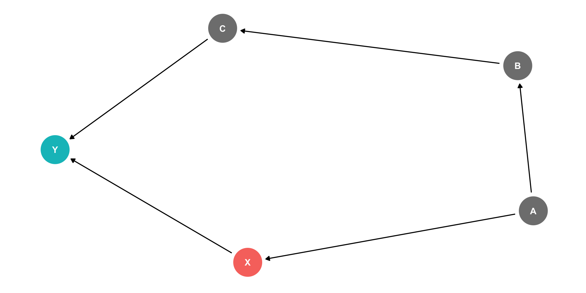
Backdoor path: \(X \leftarrow A \rightarrow B \rightarrow C \rightarrow Y\)
It is sufficient to block this backdoor by controlling either \(A\) or \(B\) or \(C\)!
Controlling II
Controlling for a single variable along a long causal path is sufficient to block that path!
Causal path: \(X \rightarrow Y\)
Backdoor path: \(X \leftarrow A \rightarrow B \rightarrow C \rightarrow Y\)
It is sufficient to block this backdoor by controlling either \(A\) or \(B\) or \(C\)!
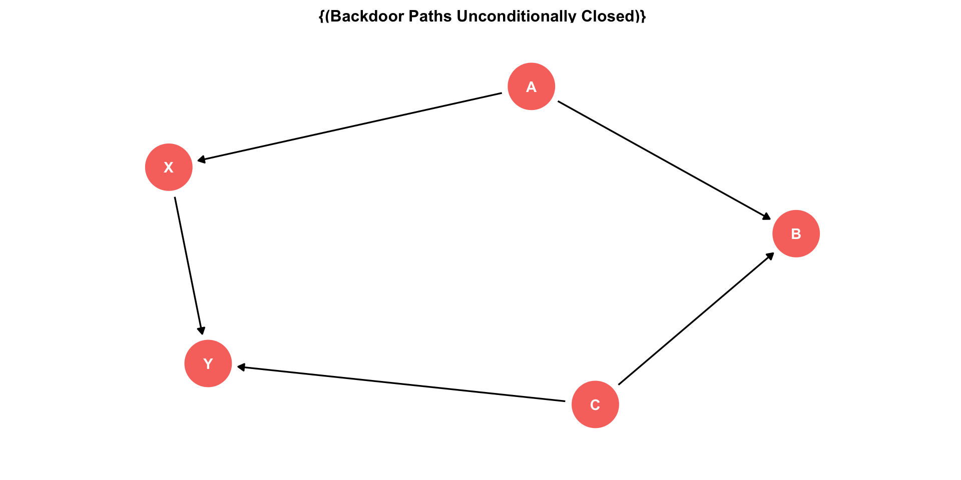
The Back Door Criterion
To identify the causal effect of \(X \rightarrow Y\):
“Back-door criterion”: control for the minimal amount of variables sufficient to ensure that no open back-door exists between \(X\) and \(Y\)
Example: in this DAG, control for \(Z\)

The Back Door Criterion
- Implications of the Back-door criterion:
- You only need to control for the variables that keep a back-door open, not all other variables!
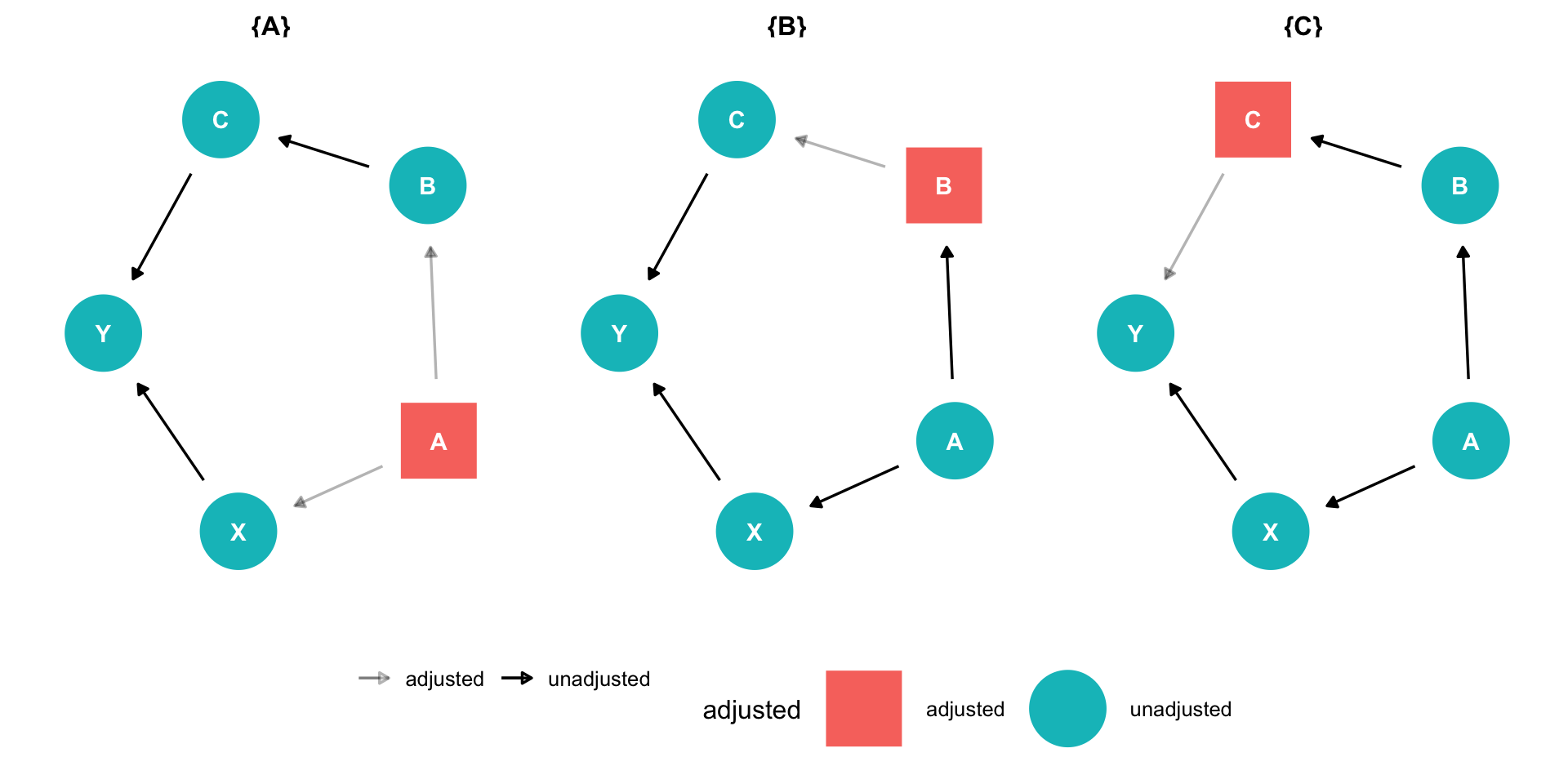
Example:
- \(X \rightarrow Y\) (front-door)
- \(X \leftarrow A \rightarrow B \rightarrow Y\) (back-door)
The Back Door Criterion
- Implications of the Back-door criterion:
- You only need to control for the variables that keep a back-door open, not all other variables!
Example:
\(X \rightarrow Y\) (front-door)
\(X \leftarrow A \rightarrow B \rightarrow Y\) (back-door)
Need only control for \(A\) or \(B\) to block the back-door path
\(C\) and \(Z\) have no effect on \(X\), and therefore we don’t need to control for them!
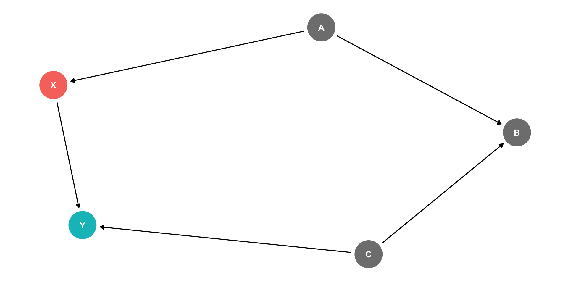
The Back Door Criterion: Colliders
- Exception: the case of a “collider”
- If arrows “collide” at a node, that node is automatically blocking the pathway, do not control for it!
- Controlling for a collider would open the path and add bias!
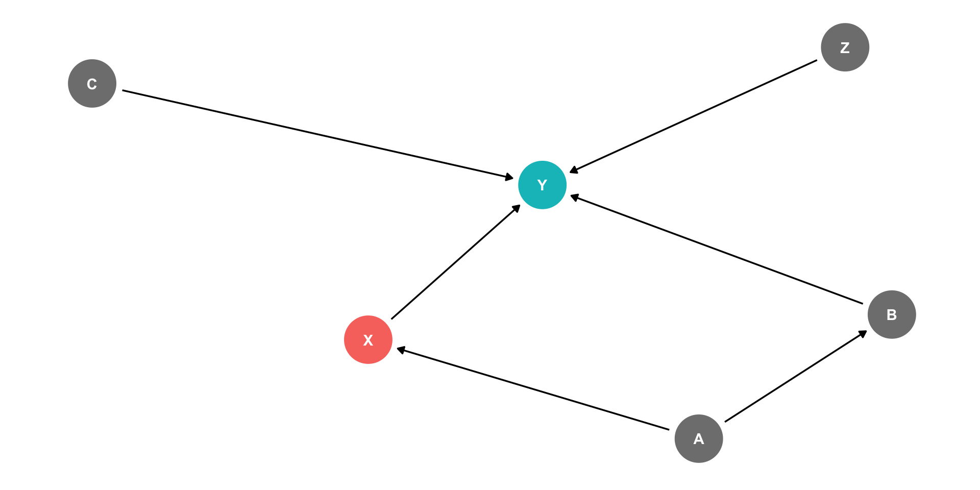
Example:
- \(X \rightarrow Y\) (front-door)
- \(X \leftarrow A \rightarrow B \leftarrow C \rightarrow Y\) (back-door, but blocked by B!)
The Back Door Criterion: Colliders
- Exception: the case of a “collider”
- If arrows “collide” at a node, that node is automatically blocking the pathway, do not control for it!
- Controlling for a collider would open the path and add bias!
Example:
- \(X \rightarrow Y\) (front-door)
- \(X \leftarrow A \rightarrow B \leftarrow C \rightarrow Y\) (back-door, but blocked by B!)
- Don’t need to control for anything here!
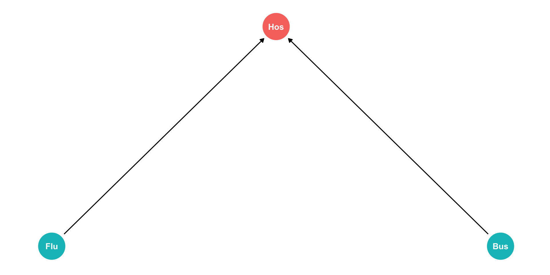
The Back Door Criterion: Colliders Example
Are you less likely to get the flu if you are hit by a bus?
\(Flu\): getting the flu
\(Bus\): being hit by a bus
\(Hos\): being in the hospital
Both \(Flu\) and \(Bus\) send you to \(Hos\) (arrows)
Conditional on being in \(Hos\), negative correlation between \(Flu\) and \(Bus\) (spurious!)
The Back Door Criterion: Colliders Example
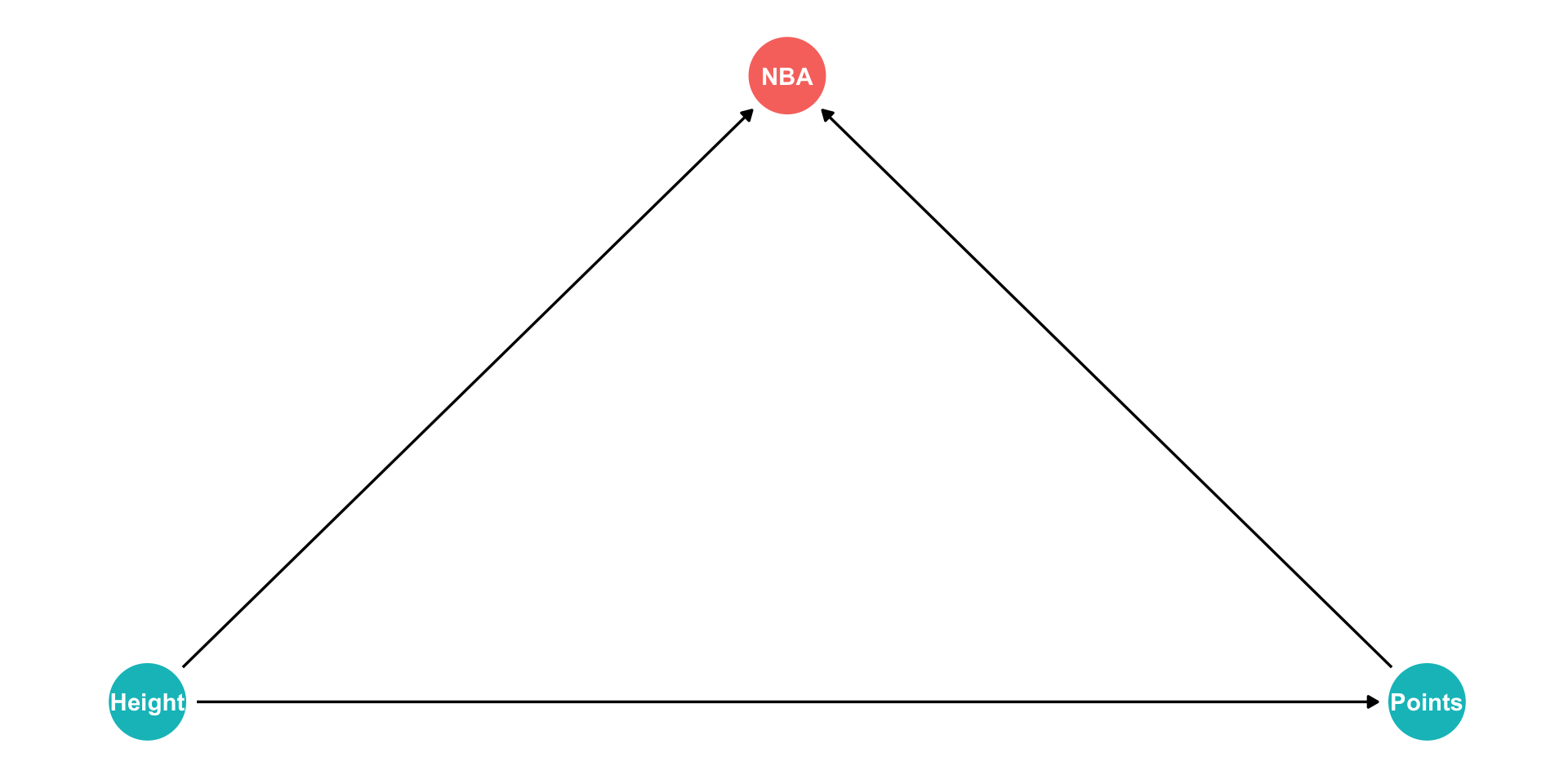
- In the NBA, apparently players’ height has no relationship to points scored?
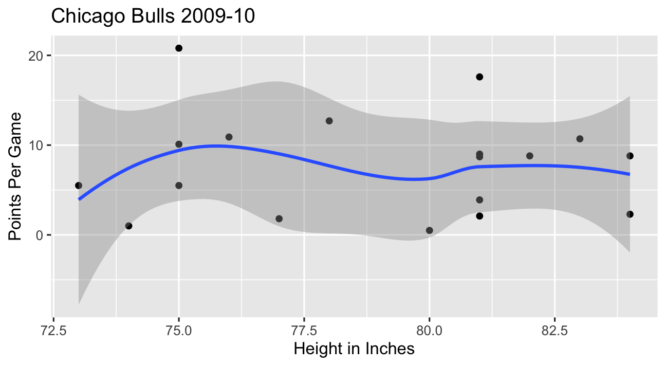
The Back Door Criterion: Colliders Example
- In the NBA, apparently players’ height has no relationship to points scored?
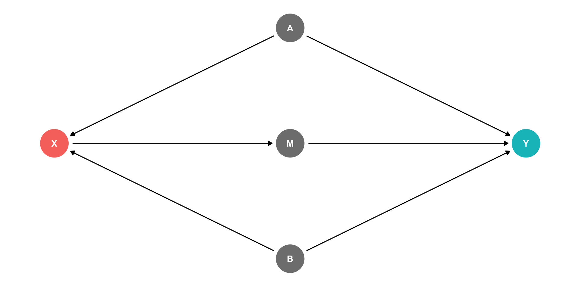
The Front Door Criterion: Mediators I
- Another case where controlling for a variable actually adds bias is if that variable is known as a “mediator”.
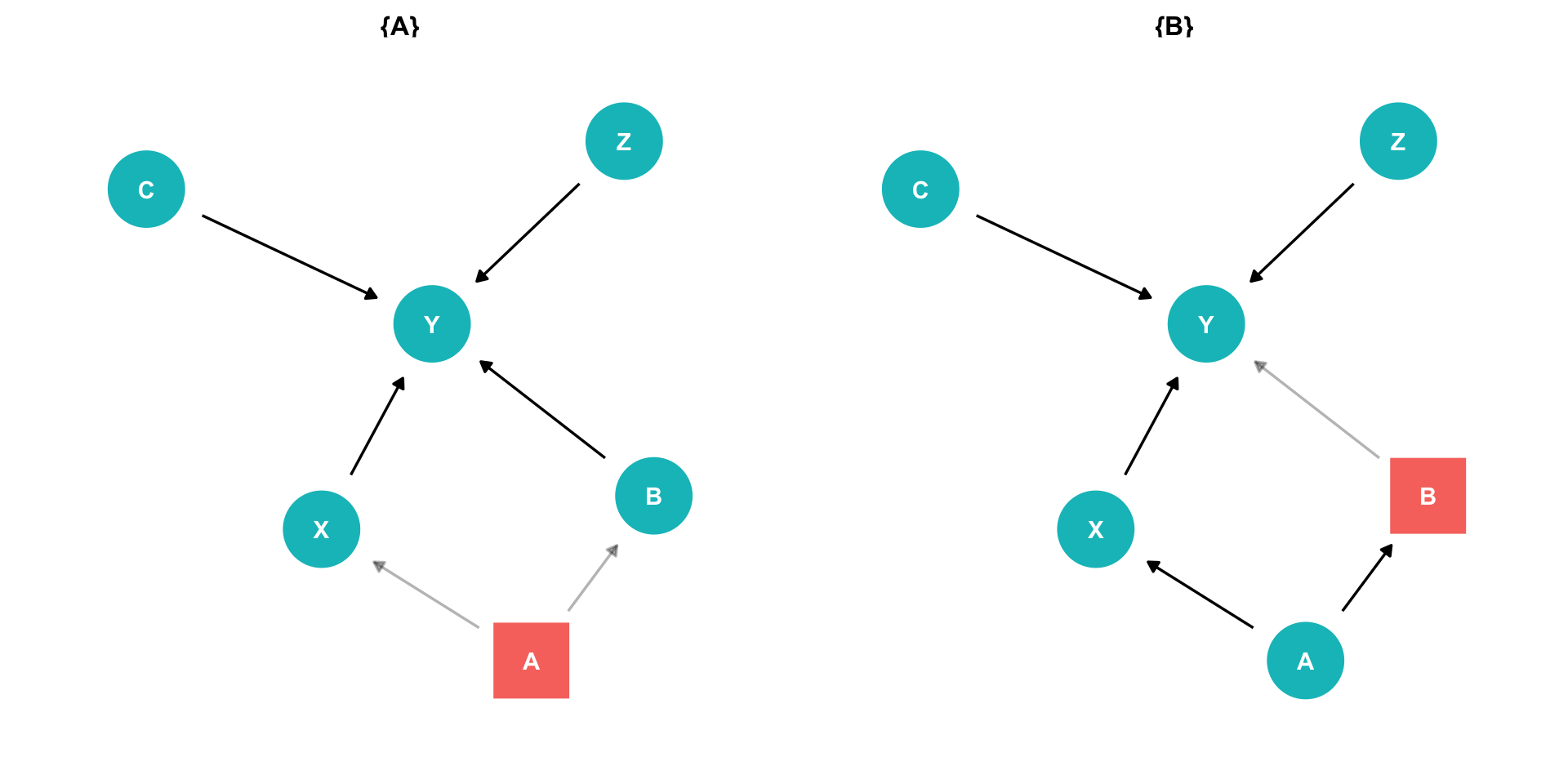
Example
\(X \rightarrow M \rightarrow Y\) (front-door)
\(X \leftarrow A \rightarrow Y\) (back-door)
\(X \leftarrow B \rightarrow Y\) (back-door)
Should we control for \(M\)?
If we did, this would block the front-door!

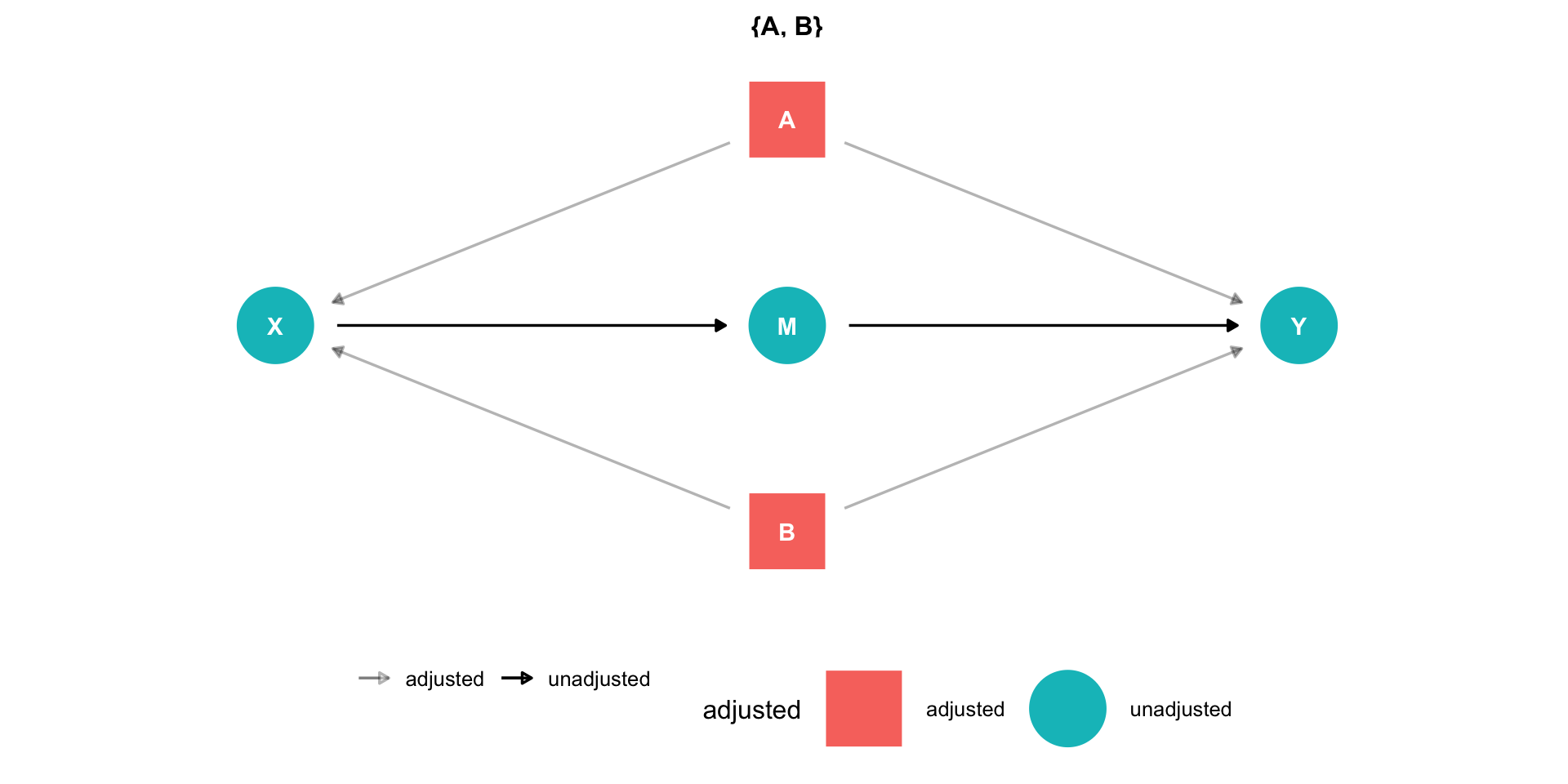
The Front Door Criterion: Mediators II
- Another case where controlling for a variable actually adds bias is if that variable is known as a “mediator”.
Example
\(X \rightarrow M \rightarrow Y\) (front-door)
\(X \leftarrow A \rightarrow Y\) (back-door)
\(X \leftarrow B \rightarrow Y\) (back-door)
If we control for \(M\), would block the front-door!
If we can estimate \(X \rightarrow M\) and \(M \rightarrow Y\) (note, no back-doors to either of these!), we can estimate \(X \rightarrow Y\)
This is the front door method
The Front Door Criterion: Mediators III
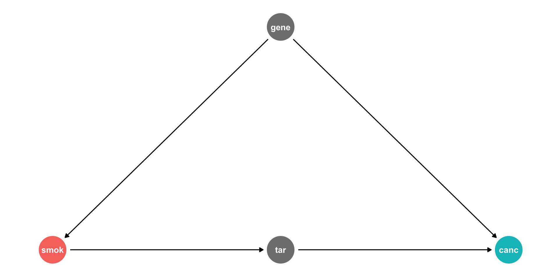
Tobacco industry claimed that \(cor(smoking, cancer)\) could be spurious due to a confounding
genethat affects both!- Smoking
geneis unobservable
- Smoking
Suppose smoking causes
tarbuildup in lungs, which causecancerWe should not control for
tar, it’s on the front-door path- This is how scientific studies can relate smoking to cancer
Summary: DAG Rules for Causal Identification
Thus, to achieve causal identification, control for the minimal amount of variables such that:
- Ensure no back-door path remains open
- Close back-door paths by controlling for any one variable along that path
- Colliders along a path automatically close that path
- Ensure no front-door path is closed
- Do not control for mediators