Omitted Variable Bias I
- Omitted variable bias (OVB) for some omitted variable \(\mathbf{Z}\) exists if two conditions are met:
1. \(\mathbf{Z}\) is a determinant of \(Y\)
- i.e. \(Z\) is in the error term, \(u_i\)
2. \(\mathbf{Z}\) is correlated with the regressor \(X\)
- i.e. \(cor(X,Z) \neq 0\)
- implies \(cor(X,u) \neq 0\)
- implies X is endogenous

Omitted Variable Bias II
Omitted variable bias makes \(X\) endogenous
Violates zero conditional mean assumption
\[\mathbb{E}(u_i|X_i)\neq 0 \implies\]
- knowing \(X_i\) tells you something about \(u_i\) (i.e. something about \(Y\) not by way of \(X\))!
Omitted Variable Bias III
\(\hat{\beta_1}\) is biased: \(\mathbb{E}[\hat{\beta_1}] \neq \beta_1\)
\(\hat{\beta_1}\) systematically over- or under-estimates the true relationship \((\beta_1)\)
\(\hat{\beta_1}\) “picks up” both pathways:
- \(X\rightarrow Y\)
- \(X \leftarrow Z\rightarrow Y\)

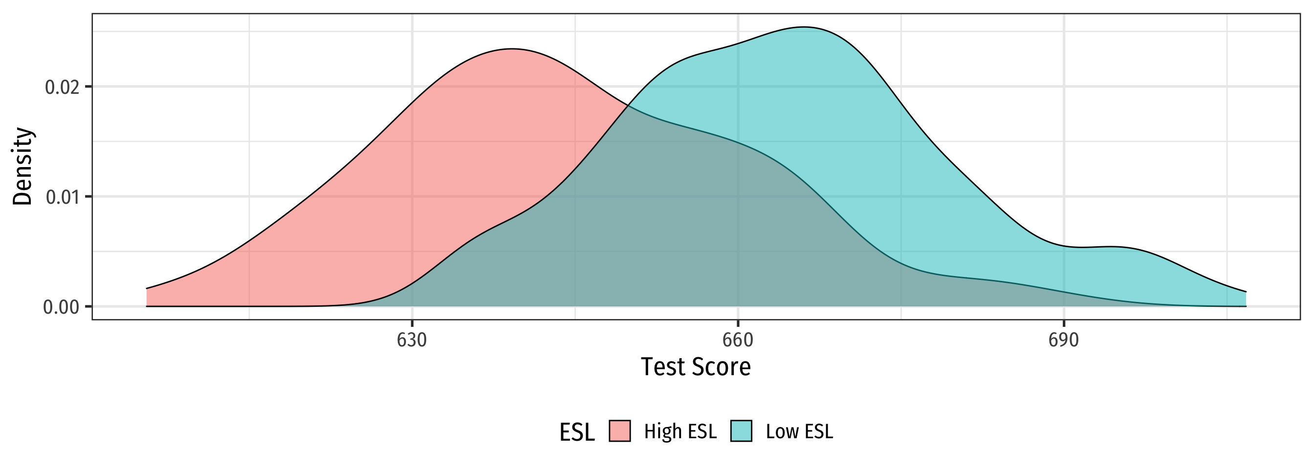
Look at Conditional Distributions II
Look at Conditional Distributions III

Look at Conditional Distributions IV
Omitted Variable Bias: Messing with Causality II
Consider an ideal random controlled trial (RCT)
Randomly assign experimental units (e.g. people, cities, etc) into two (or more) groups:
- Treatment group(s): gets a (certain type or level of) treatment
- Control group(s): gets no treatment(s)
Compare results of two groups to get average treatment effect

RCTs Neutralize Omitted Variable Bias I
School districts would be randomly assigned a student-teacher ratio
With random assignment, all factors in \(u\) (%ESL students, family size, parental income, years in the district, day of the week of the test, climate, etc) are distributed independently of class size

RCTs Neutralize Omitted Variable Bias II
Thus, \(cor(STR, u)=0\) and \(E[u|STR]=0\), i.e. exogeneity
Our \(\hat{\beta_1}\) would be an unbiased estimate of \(\beta_1\), measuring the true causal effect of STR \(\rightarrow\) Test Score
But We Rarely, if Ever, Can Do RCTs
But we didn’t run an RCT, we have observational data!
“Treatment” of having a large or small class size is NOT randomly assigned!
\(\%EL\): plausibly fits criteria of O.V. bias!
- \(\%EL\) is a determinant of Test Score
- \(\%EL\) is correlated with STR
Thus, “control” group and “treatment” group differ systematically!
- Small STR also tend to have lower \(\%EL\); large STR also tend to have higher \(\%EL\)
- Selection bias: \(cor(STR, \%EL) \neq 0\), \(E[u_i|STR_i]\neq 0\)


Another Way to Control for Variables I
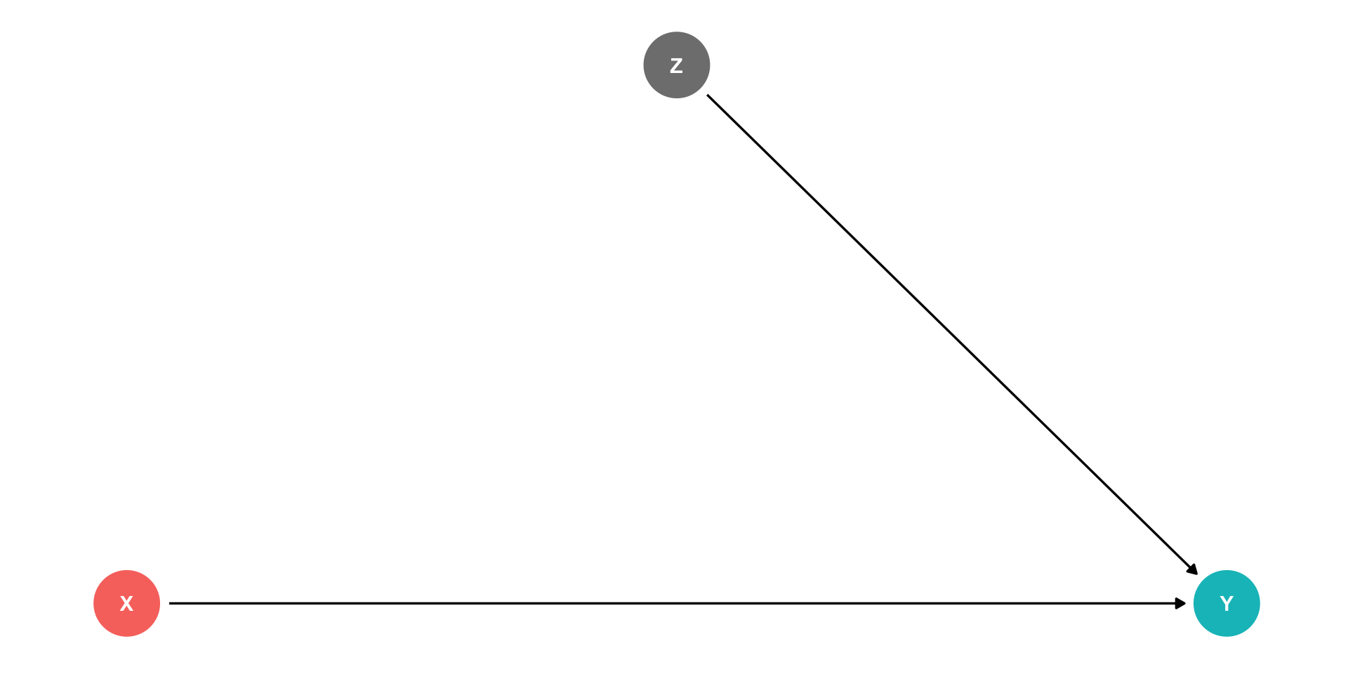
- Pathways connecting str and test score:
- str \(\rightarrow\) test score
- str \(\leftarrow\) ESL \(\rightarrow\) testscore
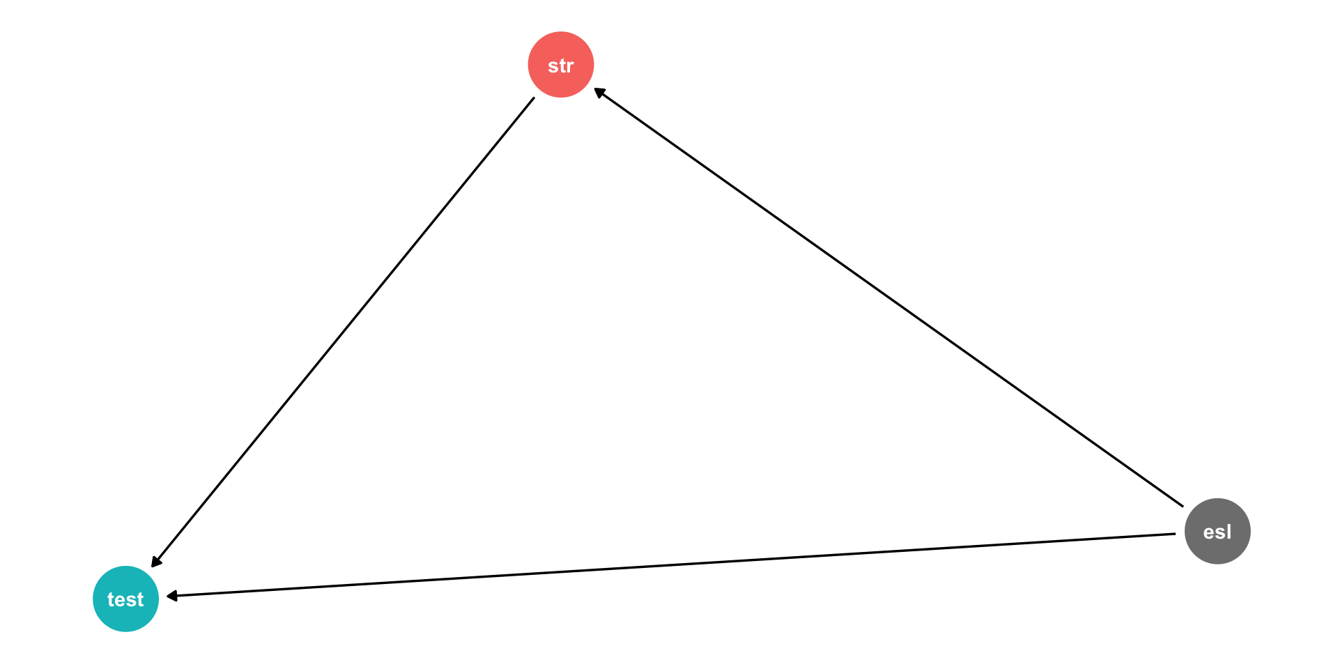
Another Way to Control for Variables II
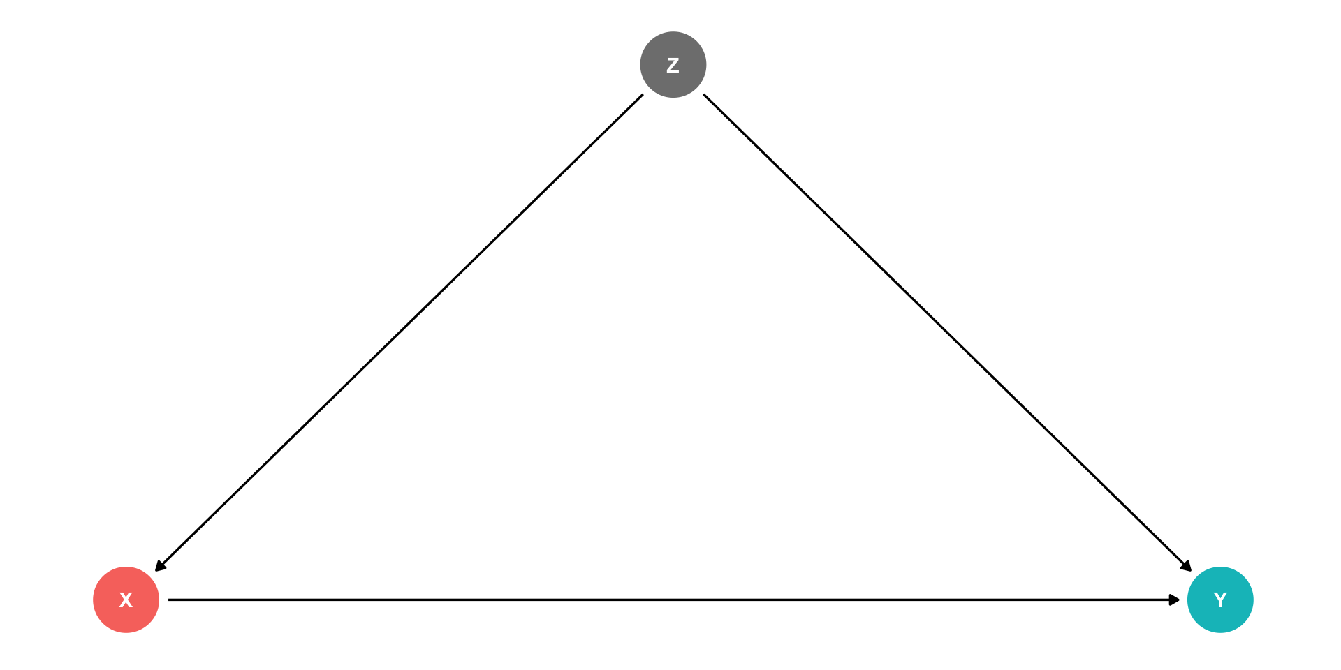
Pathways connecting str and test score:
- str \(\rightarrow\) test score
- str \(\leftarrow\) ESL \(\rightarrow\) testscore
DAG rules tell us we need to control for ESL in order to identify the causal effect of str \(\rightarrow\) test score
So now, how do we control for a variable?

Controlling for Variables
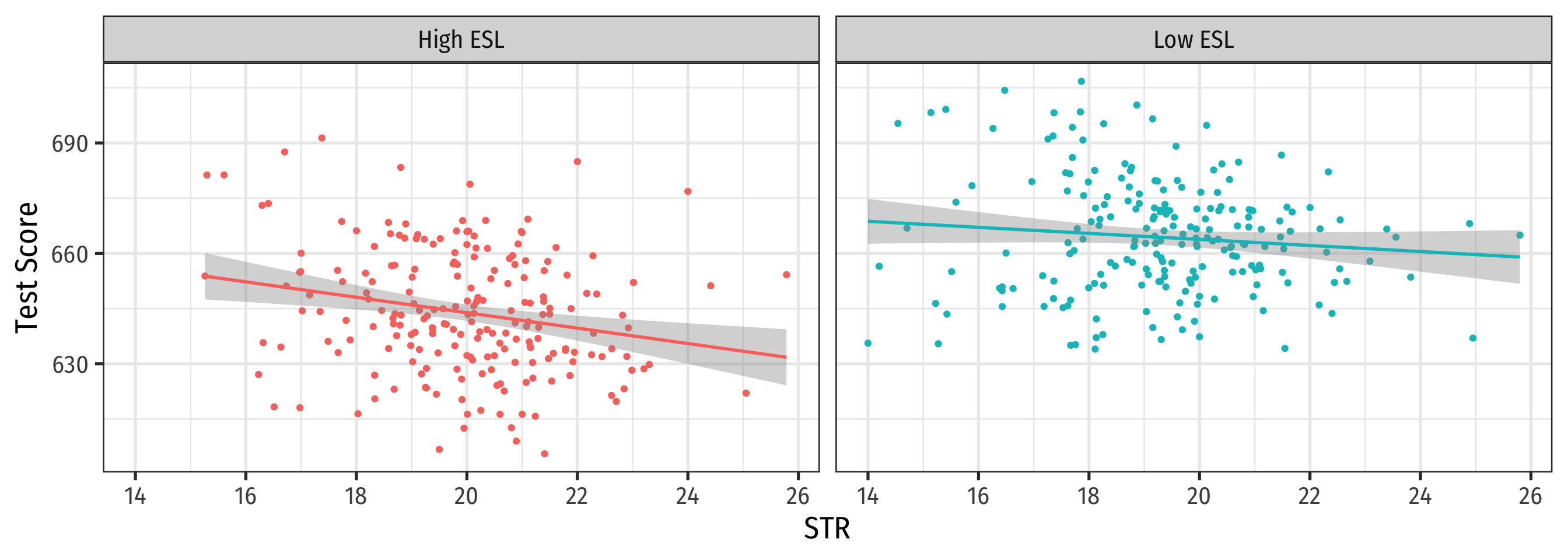
- Look at effect of STR on Test Score by comparing districts with the same %EL
- Eliminates differences in %EL between high and low STR classes
- “As if” we had a control group! Hold %EL constant
- The simple fix is just to not omit %EL!
- Make it another independent variable on the righthand side of the regression
Treatment Group
Control Group
Controlling for Variables
- Look at effect of STR on Test Score by comparing districts with the same %EL
- Eliminates differences in %EL between high and low STR classes
- “As if” we had a control group! Hold %EL constant
- The simple fix is just to not omit %EL!
- Make it another independent variable on the righthand side of the regression
Multivariate Regression Output Table
# load package
library(modelsummary)

modelsummary(models = list("Test Score" = school_reg,
                           "Test Score" = school_reg_2),
             fmt = 2, # round to 2 decimals
             output = "html",
             coef_rename = c("(Intercept)" = "Constant",
                             "str" = "STR"),
             gof_map = list(
               list("raw" = "nobs", "clean" = "n", "fmt" = 0),
               list("raw" = "r.squared", "clean" = "R<sup>2</sup>", "fmt" = 2),
               list("raw" = "rmse", "clean" = "SER", "fmt" = 2)
             ),
             escape = FALSE,
             stars = c('*' = .1, '**' = .05, '***' = 0.01)
)| Test Score | Test Score | |
|---|---|---|
| Constant | 698.93*** | 686.03*** |
| (9.47) | (7.41) | |
| STR | −2.28*** | −1.10*** |
| (0.48) | (0.38) | |
| el_pct | −0.65*** | |
| (0.04) | ||
| n | 420 | 420 |
| R2 | 0.05 | 0.43 |
| SER | 18.54 | 14.41 |
| * p < 0.1, ** p < 0.05, *** p < 0.01 |
