Categorical Variables
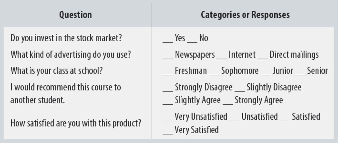
- Categorical variables place an individual into one of several possible categories
- e.g. sex, season, political party
- may be responses to survey questions
- can be quantitative (e.g. age, zip code)
- In
R:characterorfactortype datafactor\(\implies\) specific possible categories
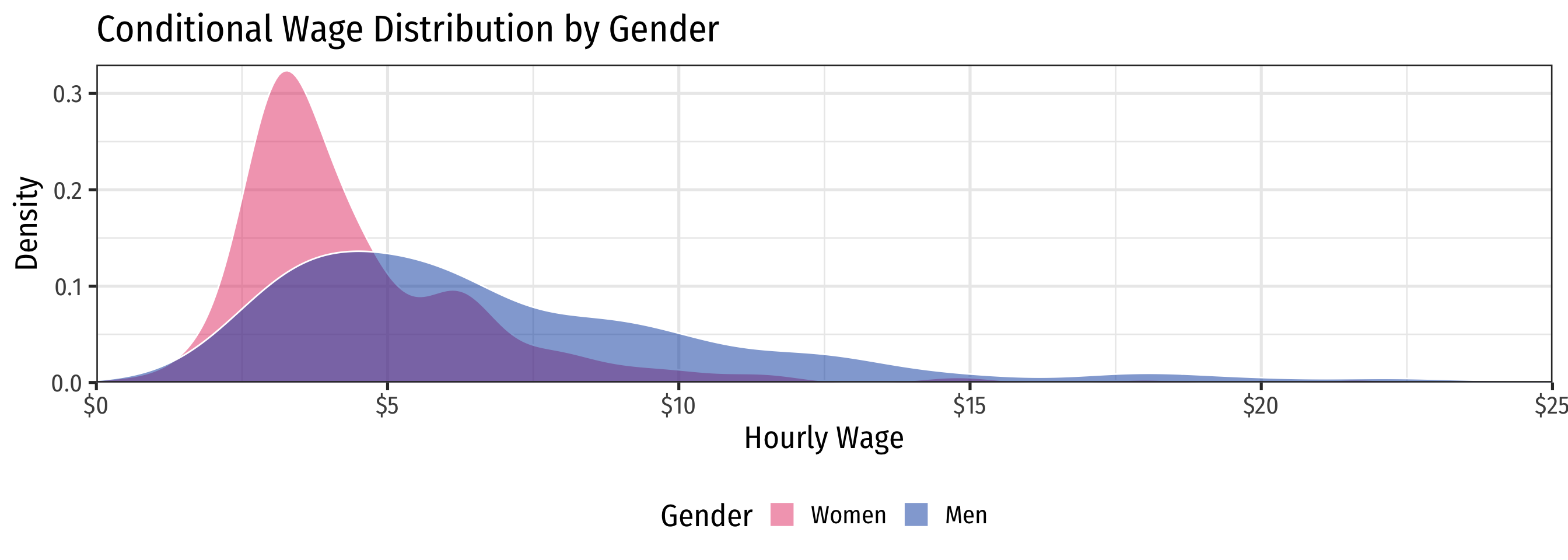
Example Research Question with Categorical Data
Example
How much higher wages, on average, do men earn compared to women?

A Difference in Group Means
Basic statistics: can test for statistically significant difference in group means with a t-test1, let:
\(Y_M\): average earnings of a sample of \(n_M\) men
\(Y_W\): average earnings of a sample of \(n_M\) women
Difference in group averages: \(d=\) \(\bar{Y}_M\) \(-\) \(\bar{Y}_W\)
The hypothesis test is:
- \(H_0: d=0\)
- \(H_1: d \neq 0\)
Plotting factors in R
- Plotting
wagevs. afactorvariable, e.g.gender(which is eitherMaleorFemale) looks like this

ggplot(data = wages)+
  aes(x = gender,
      y = wage)+
  geom_point(aes(color = gender))+
  geom_smooth(method = "lm", color = "black")+
  scale_y_continuous(labels = scales::dollar)+
  scale_color_manual(values = c("Female" = "#e64173", "Male" = "#0047AB"))+
  labs(x = "Gender",
       y = "Wage")+
  guides(color = "none")+ # hide legend
  theme_bw(base_family = "Fira Sans Condensed",
base_size = 20)- Effectively
Rtreats values of a factor variable as integers (e.g."Female"= 0,"Male"= 1)
- Let’s make this more explicit by making a dummy variable to stand in for gender
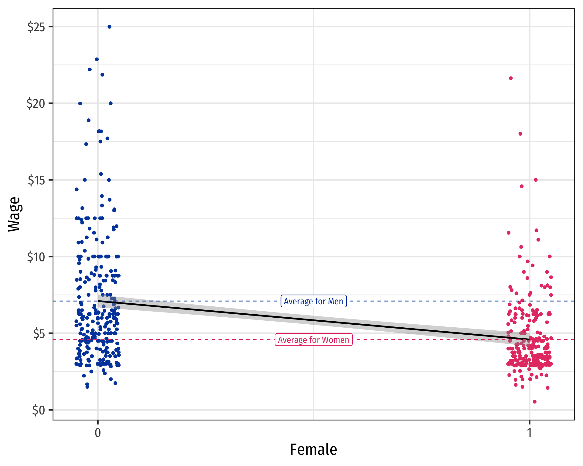
Comparing Groups in Regression: Scatterplot
ggplot(data = wages)+
  aes(x = as.factor(female),
      y = wage)+
  geom_point(aes(color = gender))+
  geom_smooth(method = "lm", color = "black")+
  scale_y_continuous(labels = scales::dollar)+
  scale_color_manual(values = c("Female" = "#e64173", "Male" = "#0047AB"))+
  labs(x = "Female",
       y = "Wage")+
  guides(color = "none")+ # hide legend
  theme_bw(base_family = "Fira Sans Condensed",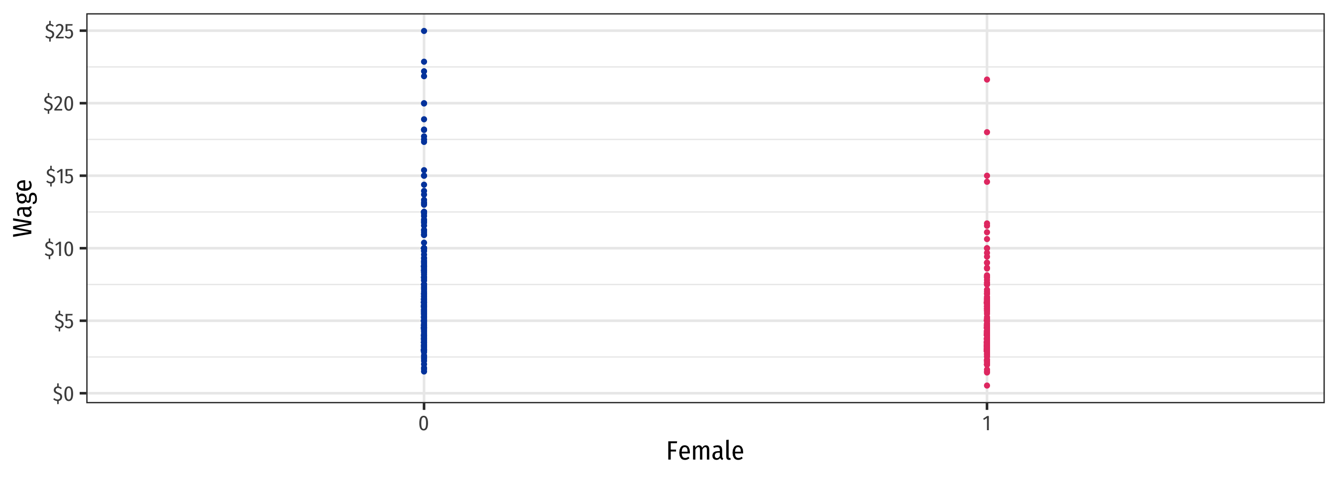
base_size = 20)- Hard to see relationships because of overplotting . . .
Comparing Groups in Regression: Scatterplot

ggplot(data = wages)+
  aes(x = as.factor(female),
      y = wage)+
  geom_jitter(aes(color = gender),
              width=0.05,
              seed = 2)+
  geom_smooth(method = "lm", color = "black")+
  scale_y_continuous(labels = scales::dollar)+
  scale_color_manual(values = c("Female" = "#e64173", "Male" = "#0047AB"))+
  labs(x = "Female",
       y = "Wage")+
  guides(color = "none")+ # hide legend
  theme_bw(base_family = "Fira Sans Condensed",
base_size = 20)- Tip: use
geom_jitter()instead ofgeom_point()to randomly nudge points!- Only used for plotting, does not affect actual data, regression, etc.
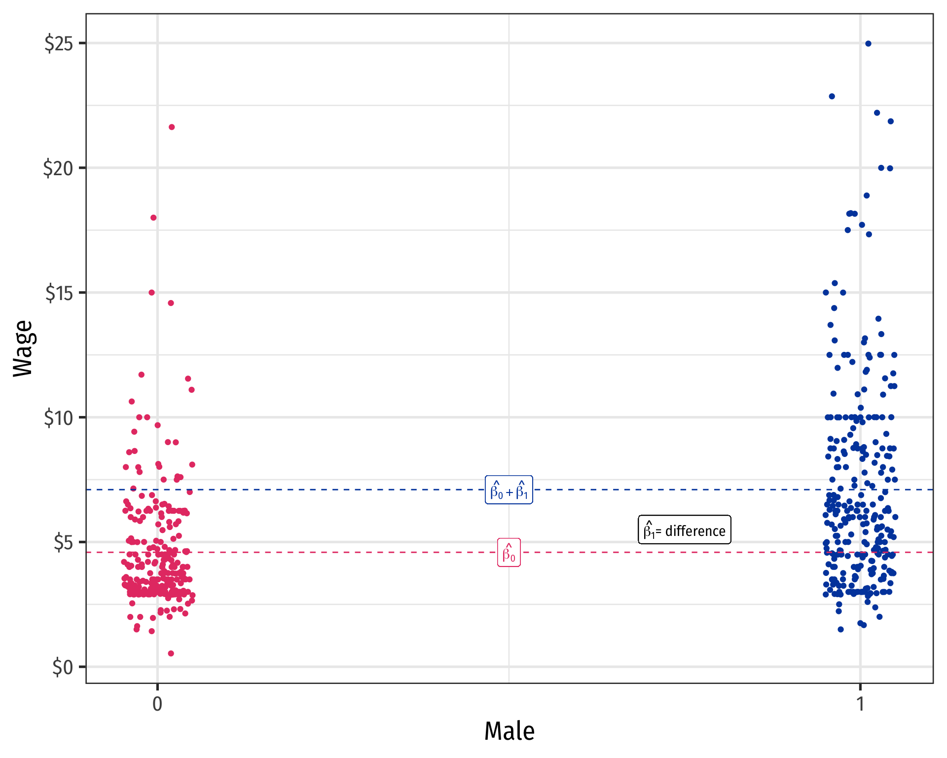
Comparing Groups in Regression: Scatterplot
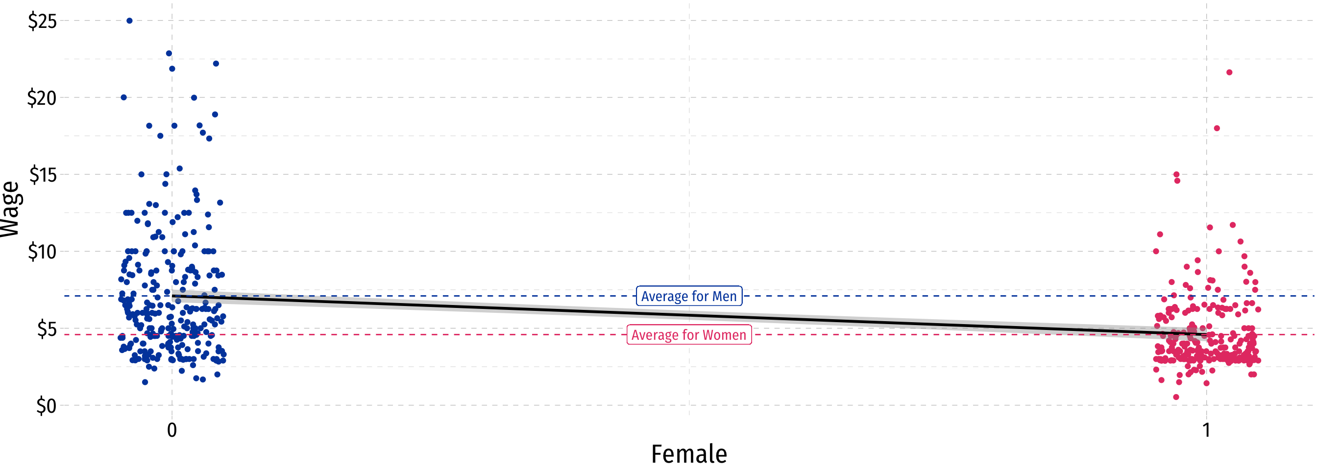
\[\widehat{Wage}_i=\hat{\beta_0}+\hat{\beta_1} \, Female_i\]
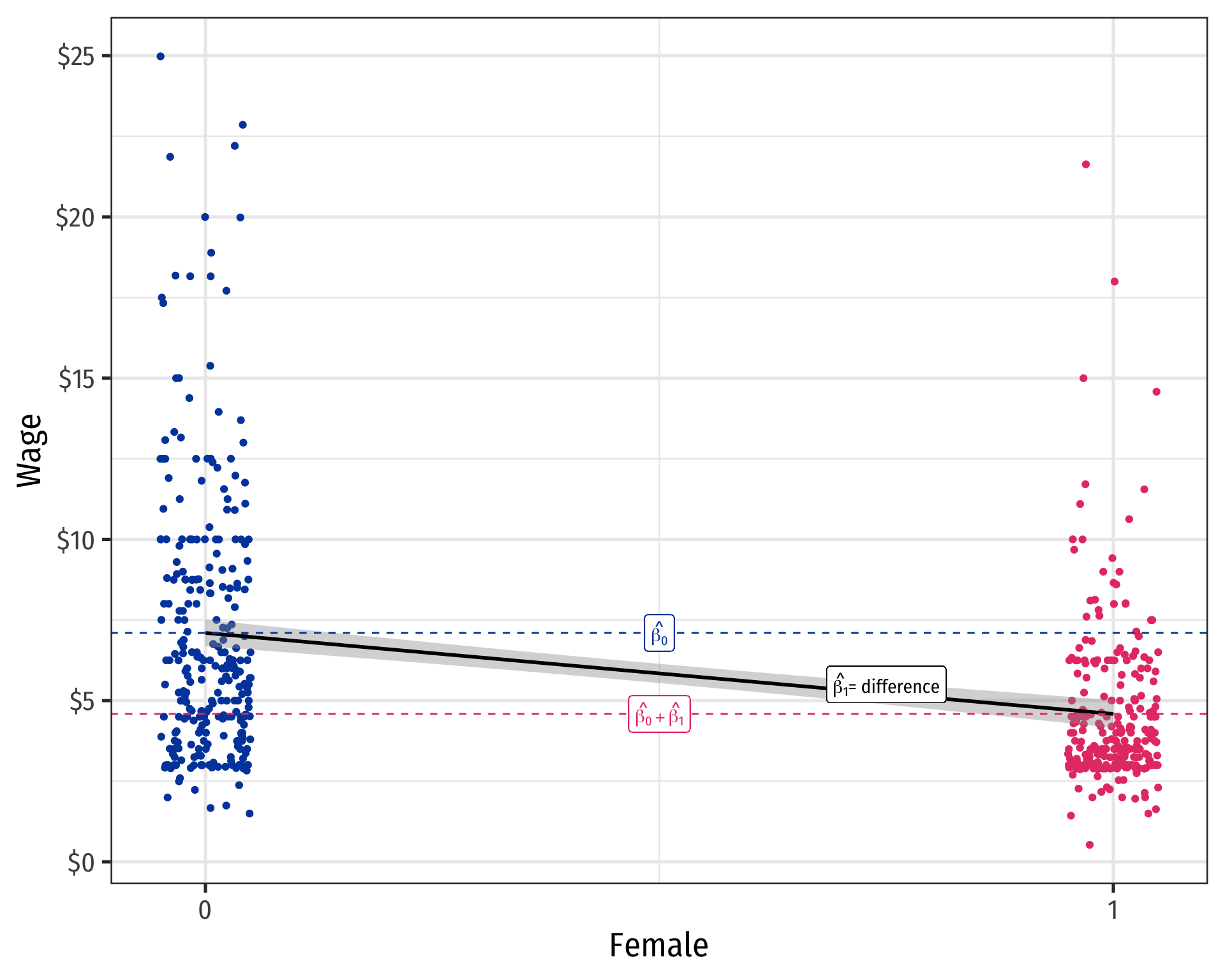
Comparing Groups in Regression: Scatterplot
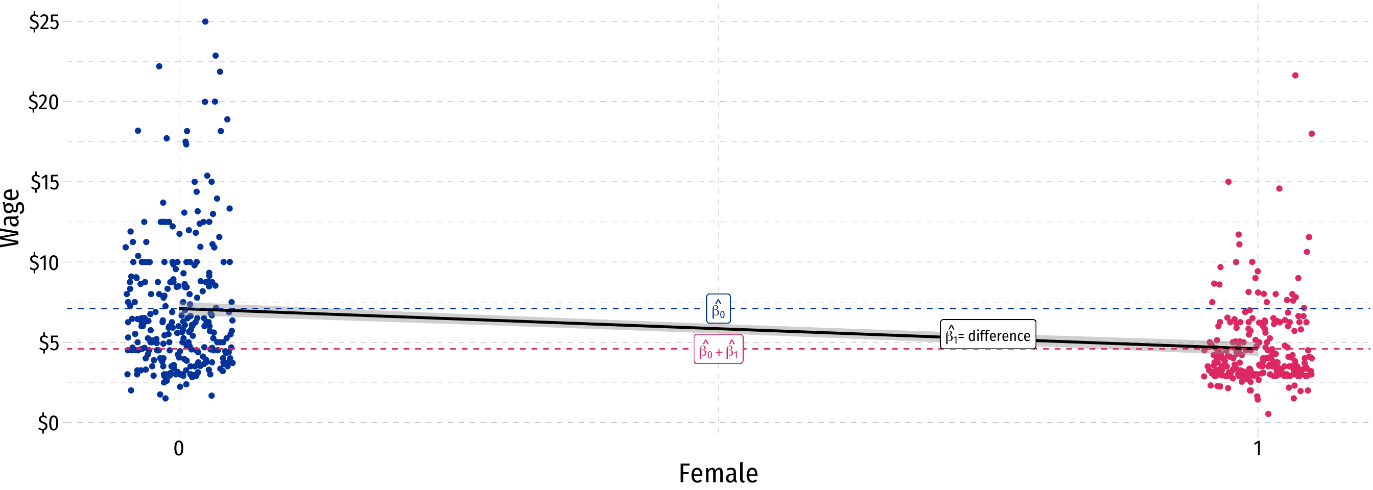
\[\widehat{Wage}_i=\hat{\beta_0}+\hat{\beta_1} \, Female_i\]
Visualize Differences
Scatterplot with Male
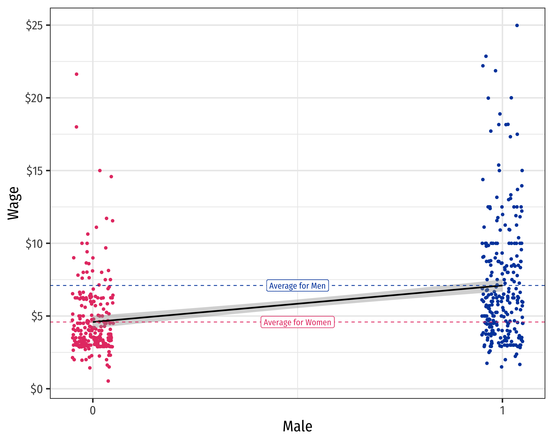
Scatterplot & Regression Line with Male
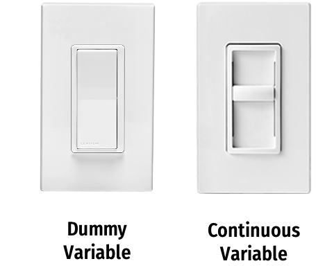
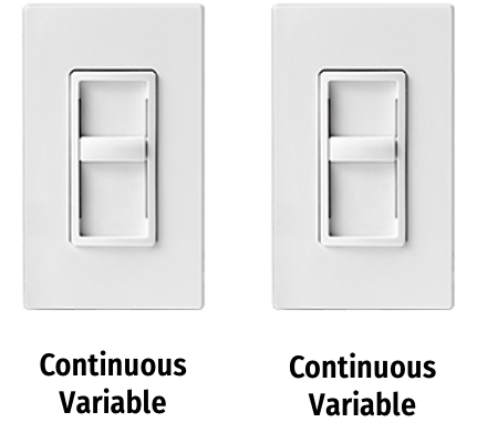
Sliders and Switches

- Marginal effect of dummy variable: effect on \(Y\) of going from 0 to 1
- Marginal effect of continuous variable: effect on \(Y\) of a 1 unit change in \(X\)
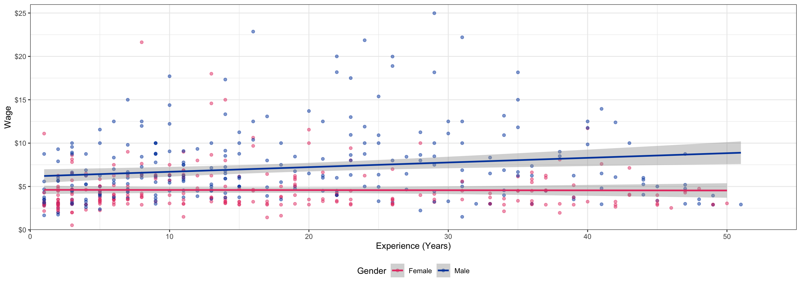
Interactions: A Dummy & Continuous Variable
- Does the marginal effect of the continuous variable on \(Y\) change depending on whether the dummy is “on” or “off”?
Dummy-Continuous Interaction Effects as Two Regressions II

- \(D_i=0\) group:
\[\color{#D7250E}{Y_i=\hat{\beta_0}+\hat{\beta_1}X_i}\]
- \(D_i=1\) group:
\[\color{#0047AB}{Y_i=(\hat{\beta_0}+\hat{\beta_2})+(\hat{\beta_1}+\hat{\beta_3})X_i}\]
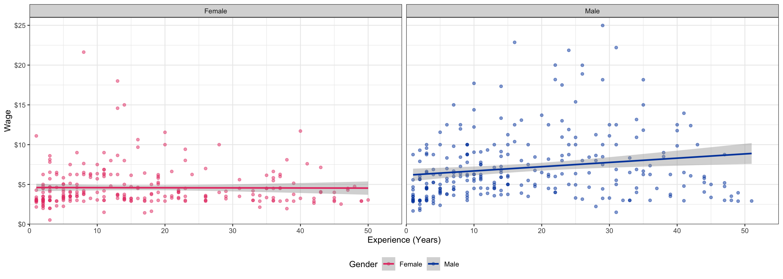
Interactions in Our Example: Scatterplot
Code
interaction_plot <- ggplot(data = wages)+
  aes(x = exper,
      y = wage,
      color = as.factor(gender))+ # make factor
  geom_point(alpha = 0.5)+
  scale_y_continuous(limits = c(0,26),
                     expand = c(0,0),
                     labels=scales::dollar)+
  scale_x_continuous(limits = c(0,55),
                     expand = c(0,0))+
  labs(x = "Experience (Years)",
       y = "Wage",
       color = "Gender")+
  scale_color_manual(values = c("Female" = "#e64173",
                                "Male" = "#0047AB")
                     )+ # setting custom colors
  theme_bw()+
  theme(legend.position = "bottom")
interaction_plot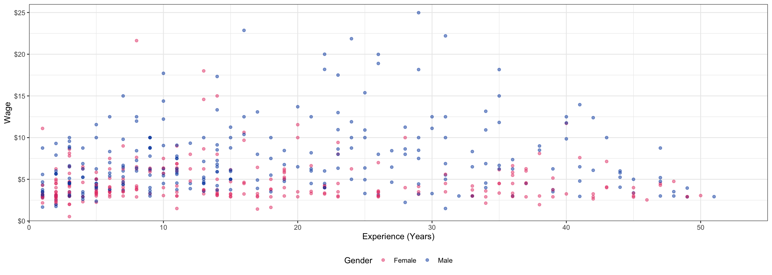
Interactions in Our Example: Scatterplot
Interactions in Our Example: Scatterplot
Interactions Between Two Dummy Variables

- Does the marginal effect on \(Y\) of one dummy going from “off” to “on” change depending on whether the other dummy is “off” or “on”?
Interactions Between Two Continuous Variables
- Does the marginal effect of \(X_1\) on \(Y\) depend on what \(X_2\) is set to?
Continuous Variables Interaction: Marginal Effects
\[\widehat{\text{wage}}_i=-2.860+0.602 \, \text{education}_i+0.047 \, \text{experience}_i+0.002\, (\text{education}_i \times \text{experience}_i)\]
Marginal Effect of Experience on Wages by Years of Education:
| Education | \(\displaystyle\frac{\Delta \text{wage}}{\Delta \text{experience}}=\hat{\beta_2}+\hat{\beta_3} \, \text{education}\) |
|---|---|
| 5 years | \(0.047+0.002(5)=0.057\) |
| 10 years | \(0.047+0.002(10)=0.067\) |
| 15 years | \(0.047+0.002(15)=0.077\) |
Marginal effect of experience \(\rightarrow\) wages increases with more education
If you want to estimate the marginal effects more precisely, and graph them, see the appendix in today’s appendix
