Linear Regression
Linear Regression
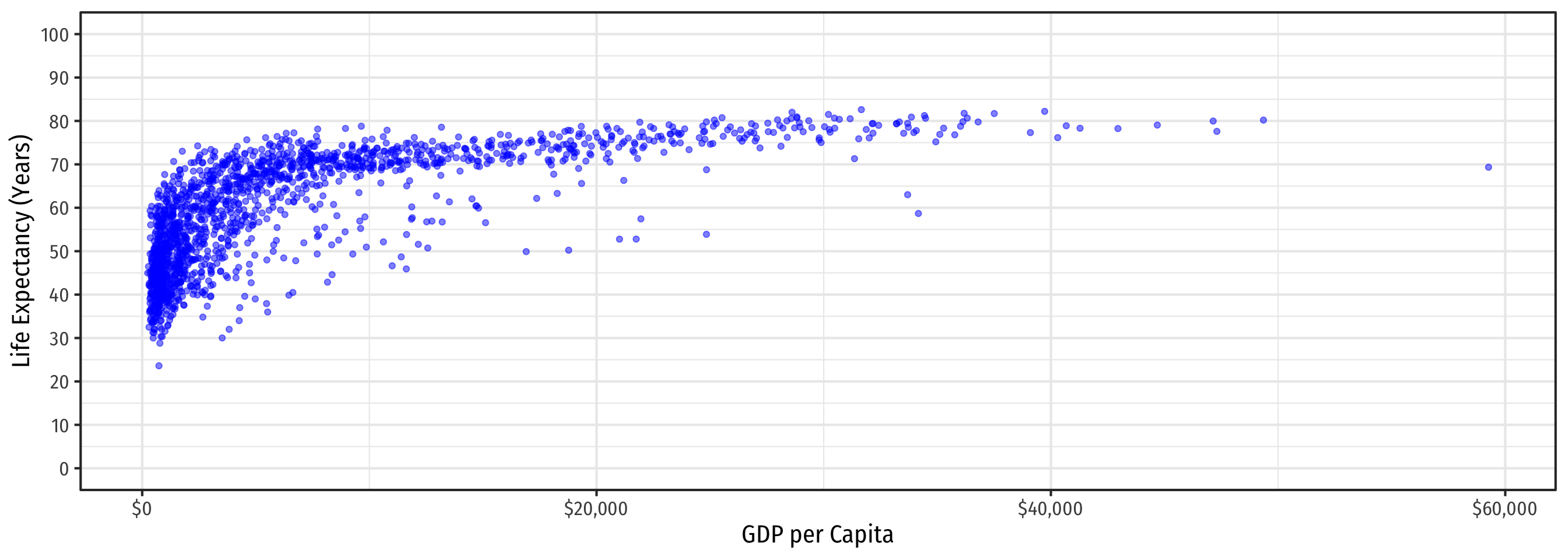
\[\color{red}{\widehat{\text{Life Expectancy}_i}=\hat{\beta_0}+\hat{\beta_1}\text{GDP}_i}\]
Linear Regression
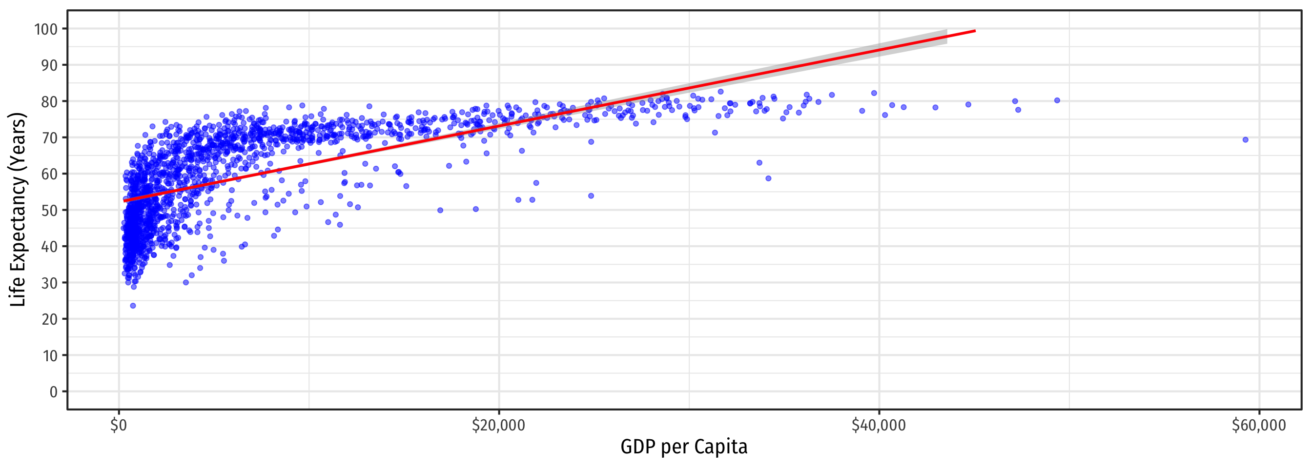
\[\color{red}{\widehat{\text{Life Expectancy}_i}=\hat{\beta_0}+\hat{\beta_1}\text{GDP}_i}\]
\[\color{green}{\widehat{\text{Life Expectancy}_i}=\hat{\beta_0}+\hat{\beta_1}\text{GDP}_i+\hat{\beta_2}\text{GDP}_i^2}\]
Linear Regression
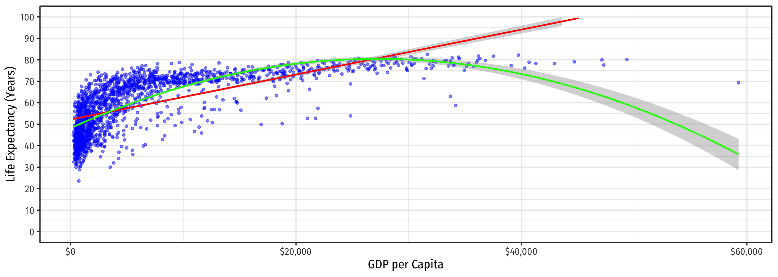
\[\color{red}{\widehat{\text{Life Expectancy}_i}=\hat{\beta_0}+\hat{\beta_1}\text{GDP}_i}\]
\[\color{green}{\widehat{\text{Life Expectancy}_i}=\hat{\beta_0}+\hat{\beta_1}\text{GDP}_i+\hat{\beta_2}\text{GDP}_i^2}\]
\[\color{orange}{\widehat{\text{Life Expectancy}_i}=\hat{\beta_0}+\hat{\beta_1}\ln \text{GDP}_i}\]
Nonlinearities Alter Marginal Effects
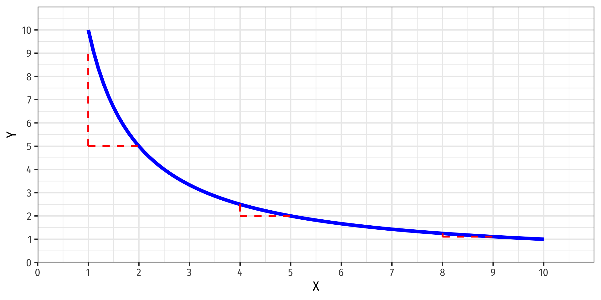
- Polynomial:
\[Y=\hat{\beta_0}+\hat{\beta_1}X+\hat{\beta_2}X^2\]
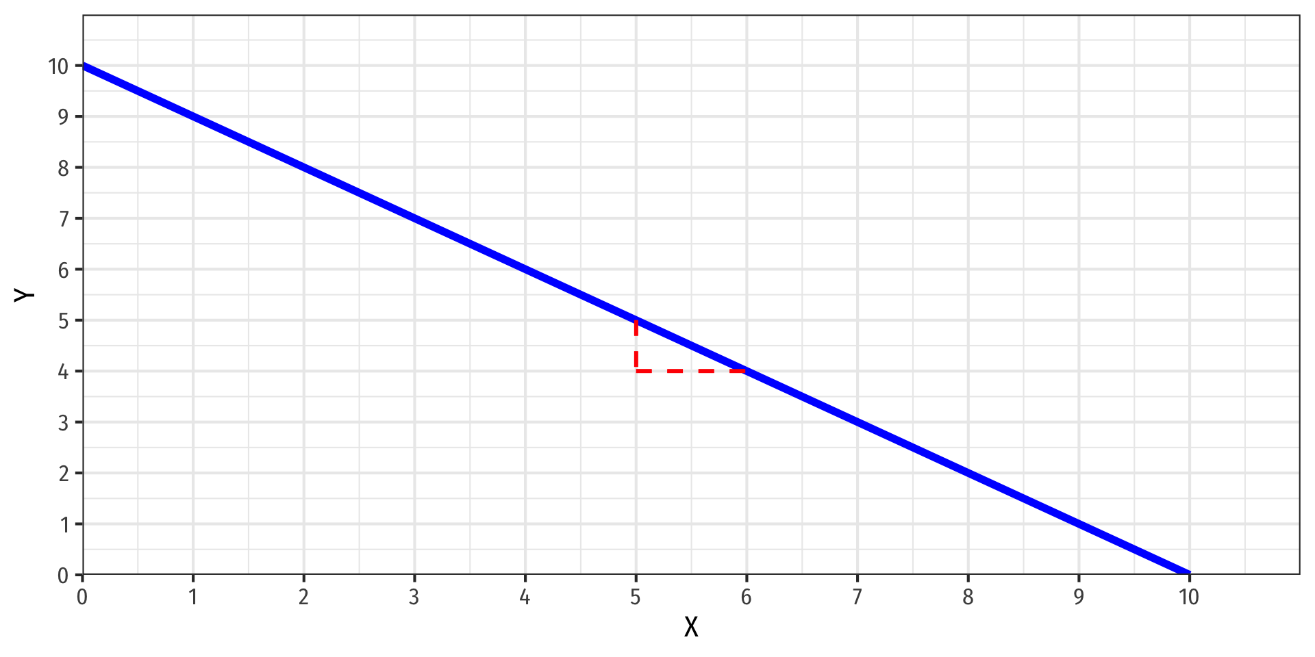
- Marginal effect, “slope” \(\left(\neq \hat{\beta_1}\right)\) depends on the value of \(X\)!
Nonlinearities Alter Marginal Effects
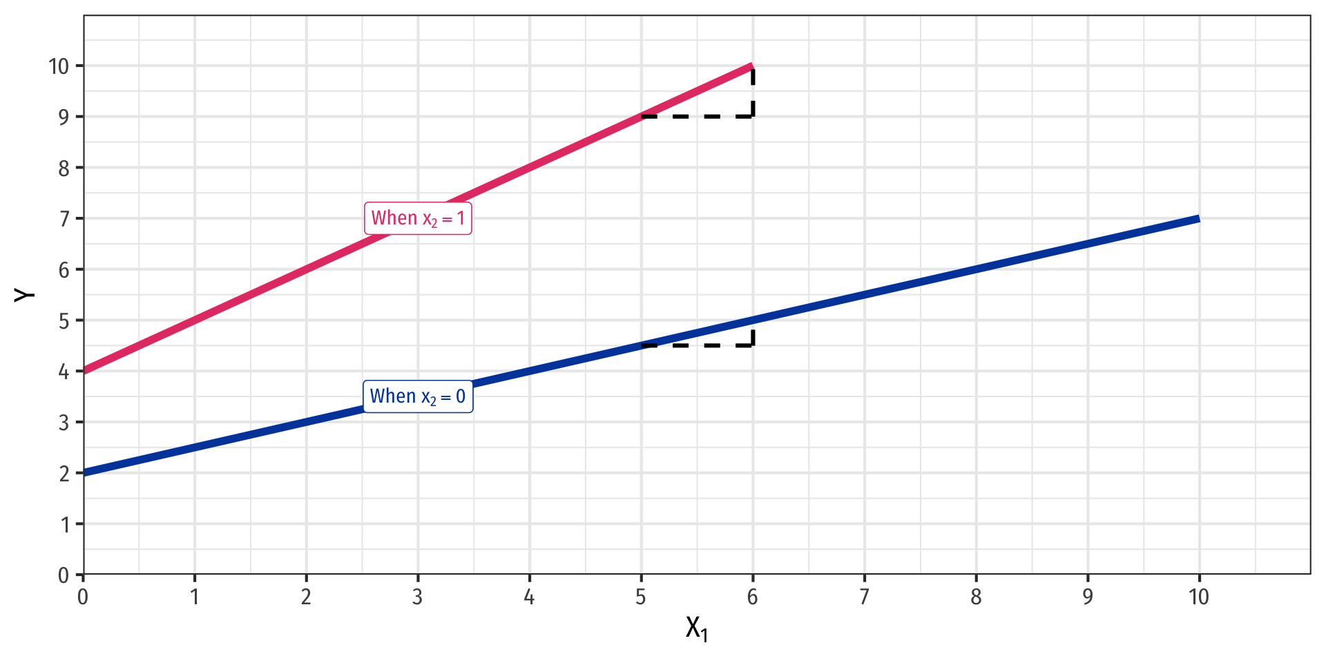
- Interaction Effect:
\[\hat{Y}=\hat{\beta_0}+\hat{\beta_1}X_1+\hat{\beta_2}X_2+\hat{\beta_3}X_1 \times X_2\]
Marginal effect, “slope” depends on the value of \(X_2\)!
Easy example: if \(X_2\) is a dummy variable:
- \(X_2=0\) (control) vs. \(X_2=1\) (treatment)
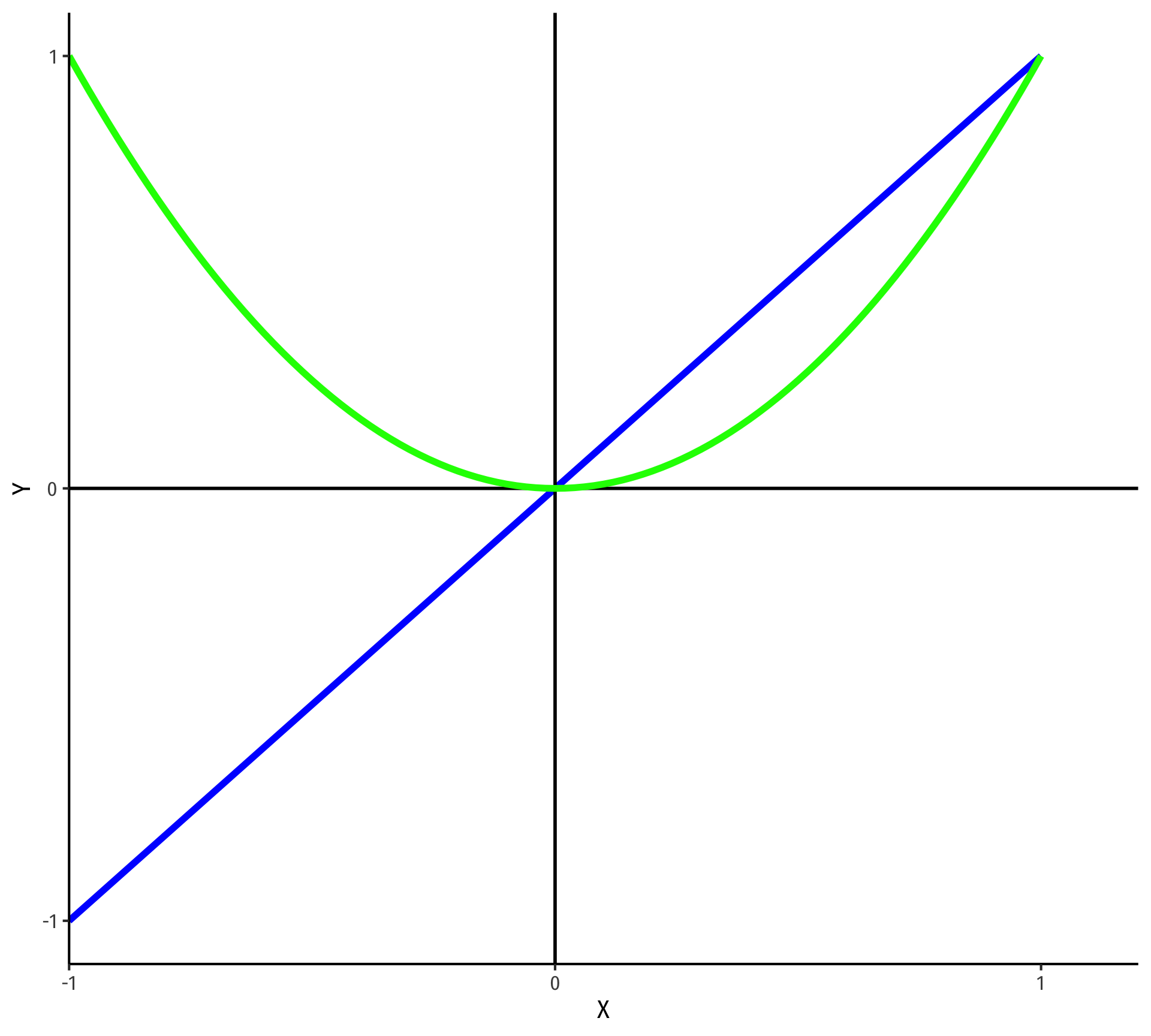
Polynomial Functions of \(X\) I
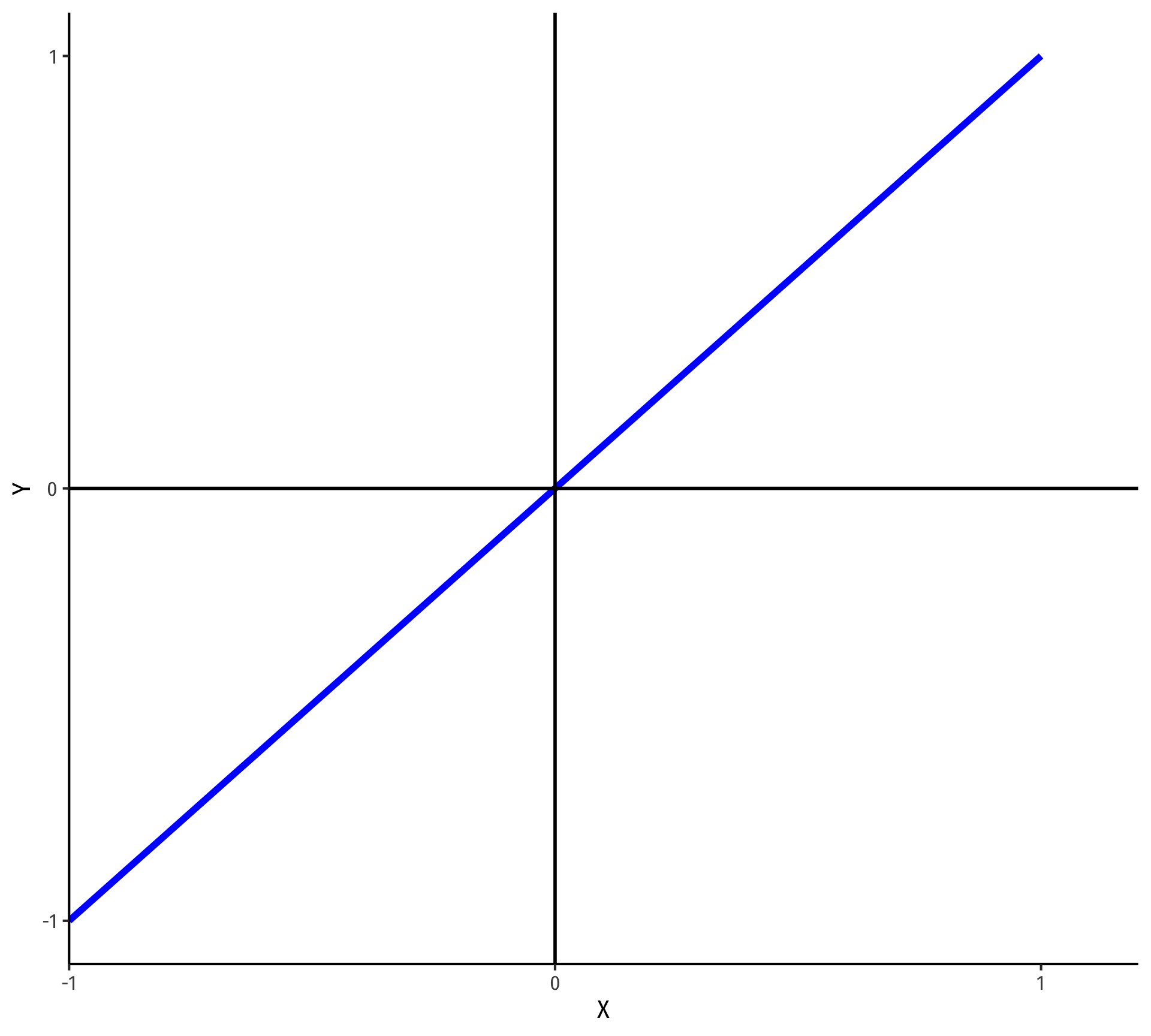
- Linear
\[\hat{Y}=\hat{\beta_0}+\hat{\beta_1}X\]
Polynomial Functions of \(X\) I
- Linear
\[\hat{Y}=\hat{\beta_0}+\hat{\beta_1}X\]
- Quadratic
\[\hat{Y}=\hat{\beta_0}+\hat{\beta_1}X+\hat{\beta_2}X^2\]
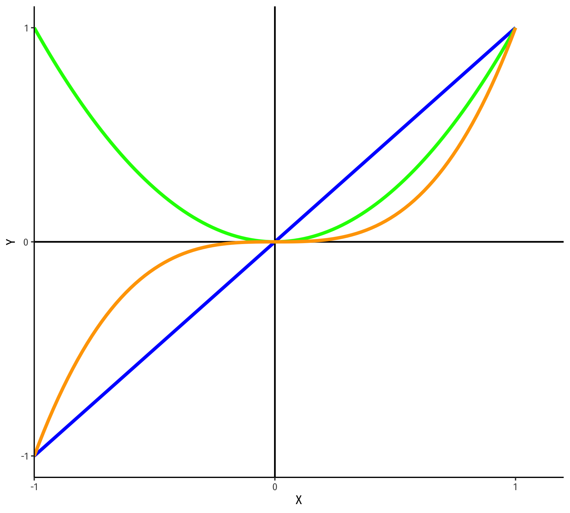
Polynomial Functions of \(X\) I
- Linear
\[\hat{Y}=\hat{\beta_0}+\hat{\beta_1}X\]
- Quadratic
\[\hat{Y}=\hat{\beta_0}+\hat{\beta_1}X+\hat{\beta_2}X^2\]
- Cubic
\[\hat{Y}=\hat{\beta_0}+\hat{\beta_1}X+\hat{\beta_2}X^2+\hat{\beta_3}X^3\]
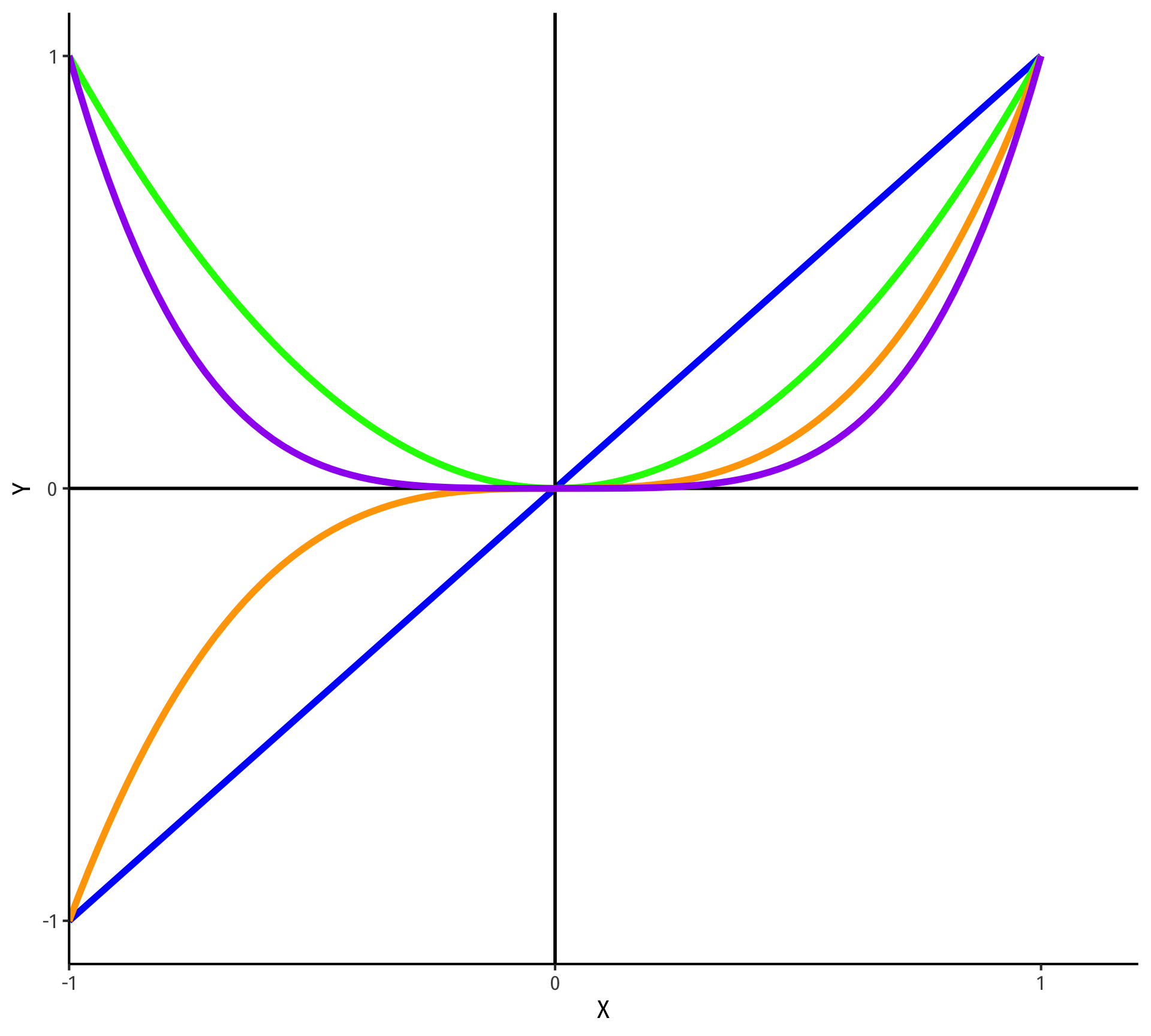
Polynomial Functions of \(X\) I
- Linear
\[\hat{Y}=\hat{\beta_0}+\hat{\beta_1}X\]
- Quadratic
\[\hat{Y}=\hat{\beta_0}+\hat{\beta_1}X+\hat{\beta_2}X^2\]
- Cubic
\[\hat{Y}=\hat{\beta_0}+\hat{\beta_1}X+\hat{\beta_2}X^2+\hat{\beta_3}X^3\]
- Quartic
\[\hat{Y}=\hat{\beta_0}+\hat{\beta_1}X+\hat{\beta_2}X^2+\hat{\beta_3}X^3+\hat{\beta_4}X^4\]
Quadratic Model: Example XII
Code
ggplot(data = gapminder)+
  aes(x = GDP_t,
      y = lifeExp)+
  geom_point(color = "blue", alpha=0.5)+
  stat_smooth(method = "lm",
              formula = y ~ x + I(x^2),
              color = "green")+
  geom_vline(xintercept = c(5,25,50),
             linetype = "dashed",
             color = "red", size = 1)+
  scale_x_continuous(labels = scales::dollar,
                     breaks = seq(0,120,10))+
  scale_y_continuous(breaks = seq(0,100,10),
                     limits = c(0,100))+
  labs(x = "GDP per Capita (in Thousands)",
       y = "Life Expectancy (Years)")+
  theme_bw(base_family = "Fira Sans Condensed",
           base_size=16)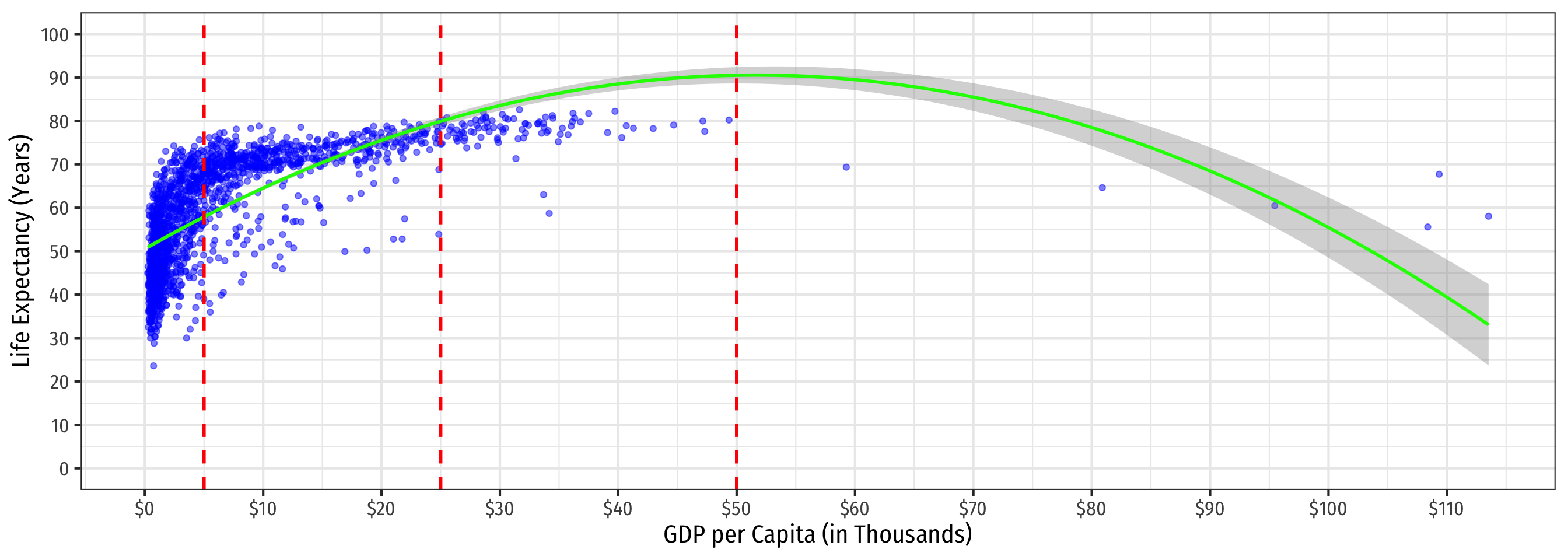
Quadratic Model: Maxima and Minima III
Code
ggplot(data = gapminder)+
  aes(x = GDP_t,
      y = lifeExp)+
  geom_point(color = "blue", alpha=0.5)+
  stat_smooth(method = "lm",
              formula = y ~ x + I(x^2),
              color = "green")+
  geom_vline(xintercept=51.67, linetype="dashed", color="red", size = 1)+
  geom_label(x=51.67, y=90, label="$51.67", color="red")+
  scale_x_continuous(labels = scales::dollar,
                     breaks = seq(0,120,10))+
  scale_y_continuous(breaks = seq(0,100,10),
                     limits = c(0,100))+
  labs(x = "GDP per Capita (in Thousands)",
       y = "Life Expectancy (Years)")+
  theme_bw(base_family = "Fira Sans Condensed",
           base_size=16)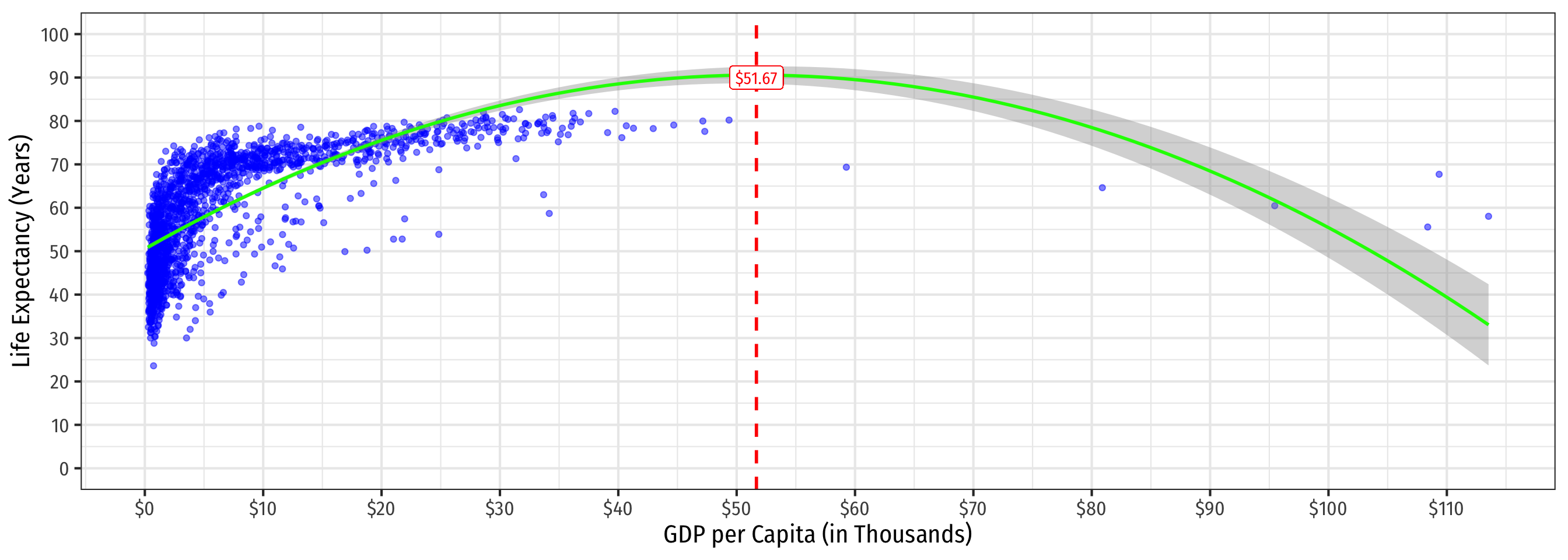
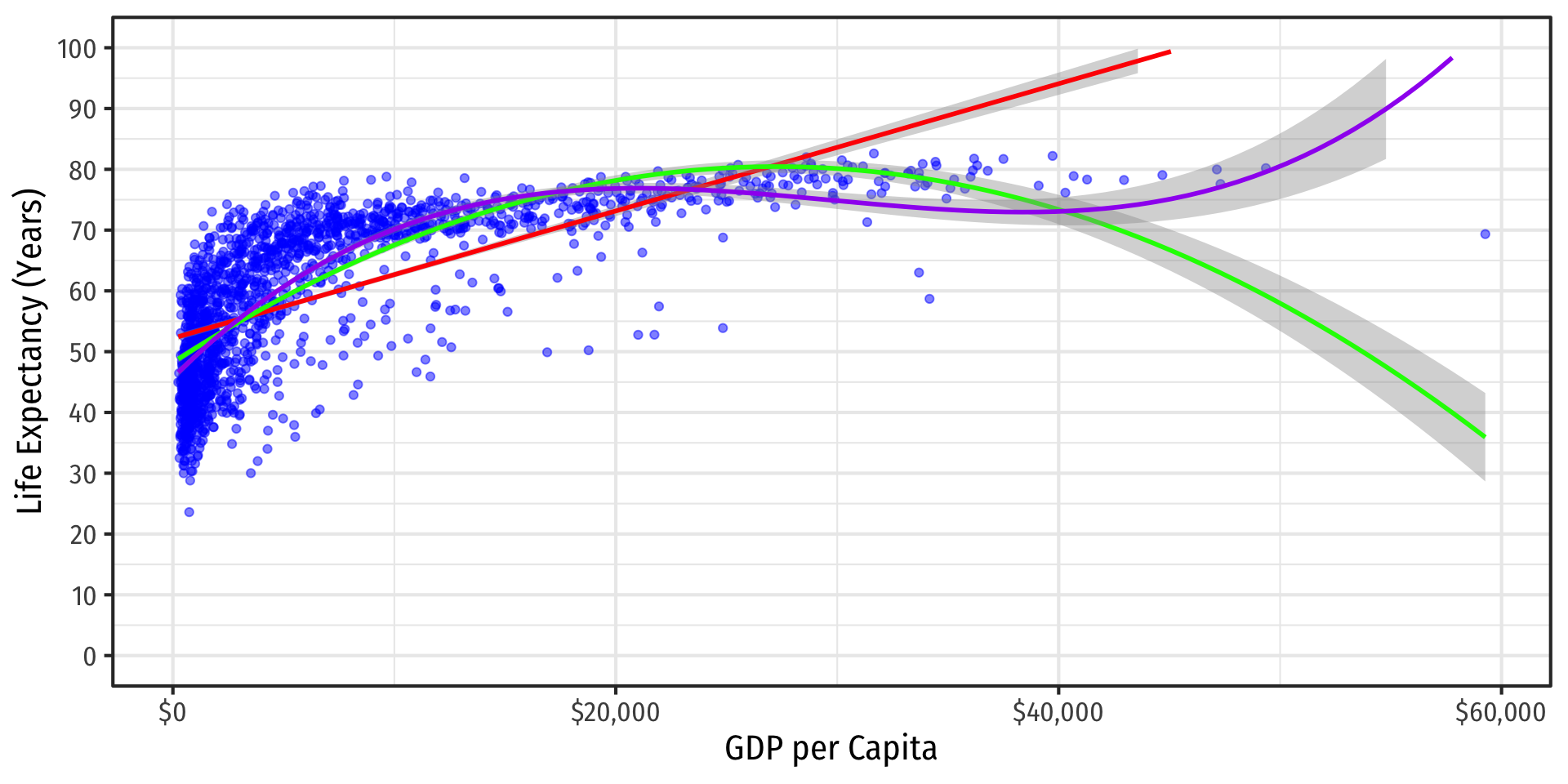
Determining Polynomials are Necessary II
- Should we keep going up in polynomials?

Determining Polynomials are Necessary II
- Should we keep going up in polynomials?
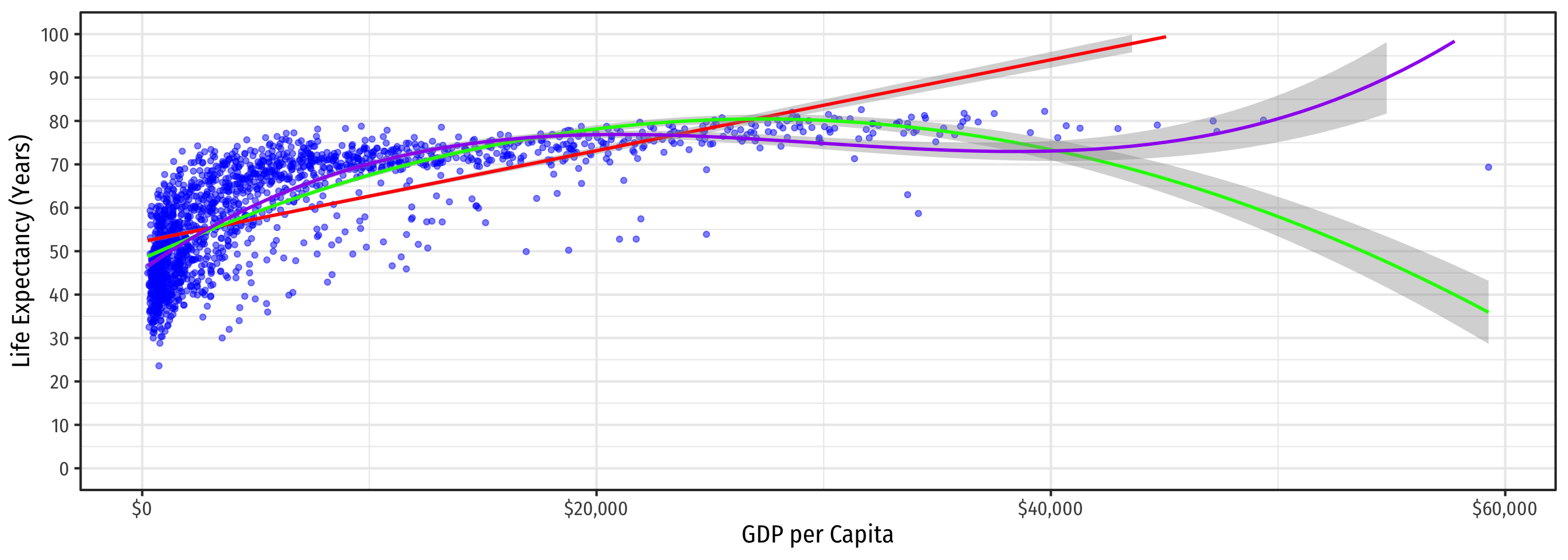
\[\color{#6A5ACD}{\widehat{\text{Life Expectancy}_i} = \hat{\beta_0}+\hat{\beta_1} GDP_i+\hat{\beta_2}GDP^2_i+\hat{\beta_3}GDP_i^3}\]
Determining Polynomials are Necessary III
In general, you should have a compelling theoretical reason why data or relationships should “change direction” multiple times
Or clear data patterns that have multiple “bends”
Recall, we care more about accurately measuring the causal effect of \(X \rightarrow Y\), rather than getting the most accurate prediction possible for \(\hat{Y}\)
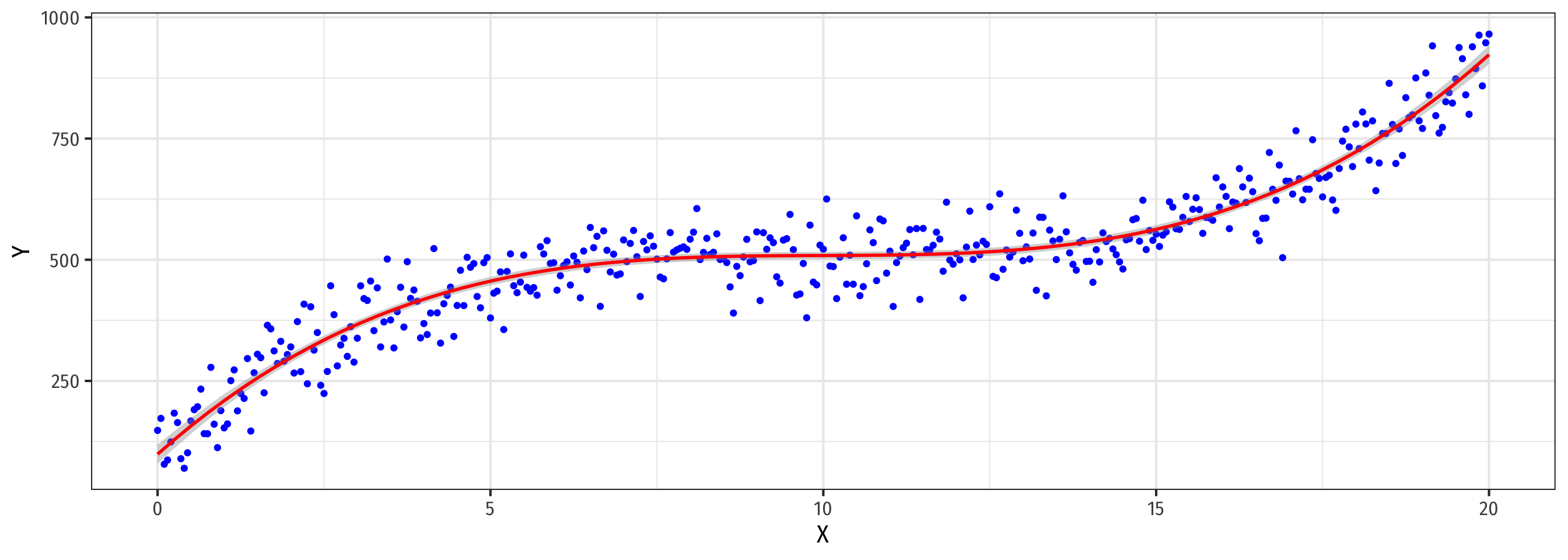
If You Kept Going…Visually
If You Kept Going…Visually
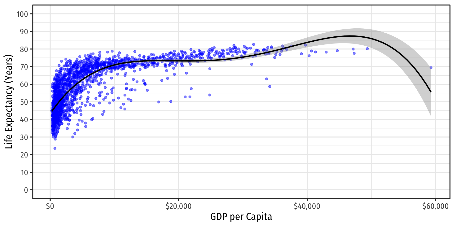
A 4th-degree polynomial
If You Kept Going…Visually
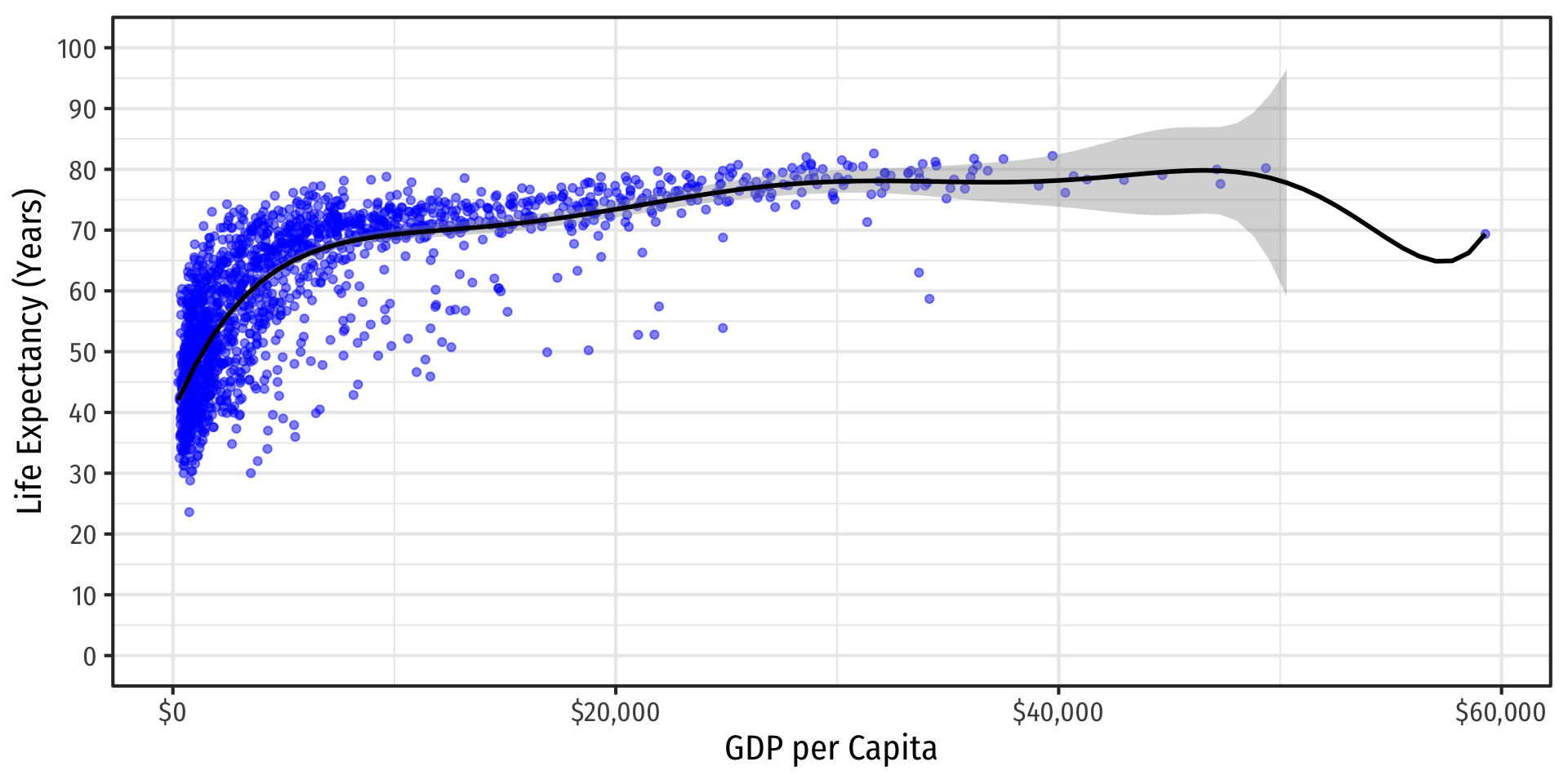
A 9th-degree polynomial
If You Kept Going…Visually
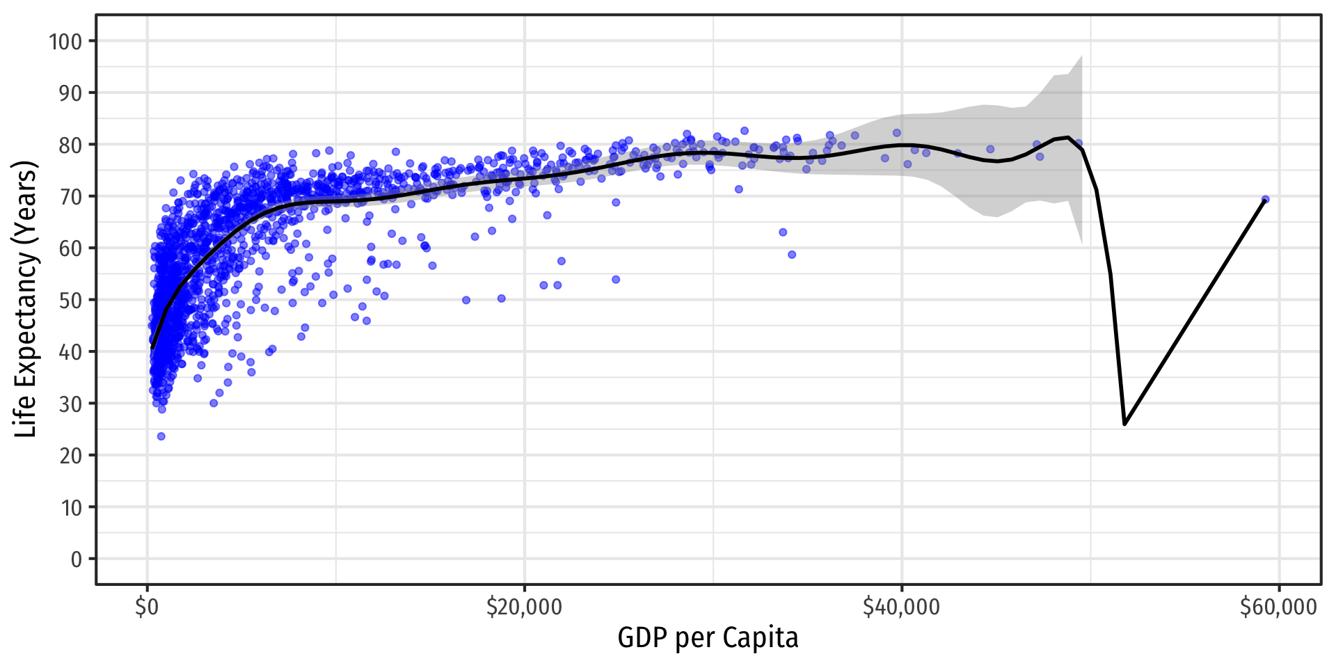
A 14th-degree polynomial
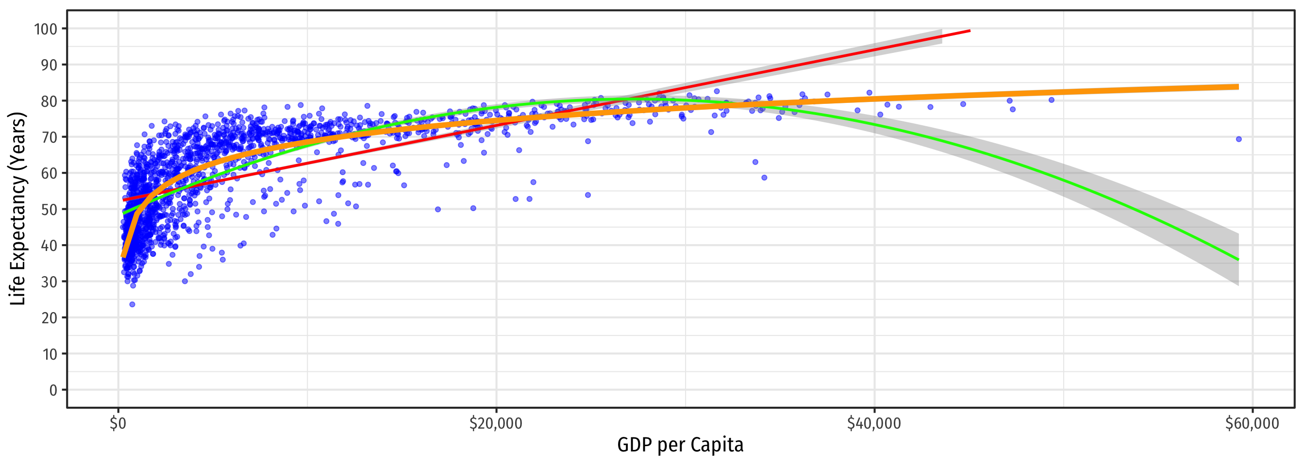
Linear Regression

\[\color{red}{\widehat{\text{Life Expectancy}_i}=\hat{\beta_0}+\hat{\beta_1}\text{GDP}_i}\]
\[\color{green}{\widehat{\text{Life Expectancy}_i}=\hat{\beta_0}+\hat{\beta_1}\text{GDP}_i+\hat{\beta_2}\text{GDP}_i^2}\]
\[\color{orange}{\widehat{\text{Life Expectancy}_i}=\hat{\beta_0}+\hat{\beta_1}\ln \text{GDP}_i}\]
Logarithmic Models
- Another useful model for nonlinear data is the logarithmic model1
- We transform either \(X\), \(Y\), or both by taking the (natural) logarithm
- Logarithmic model has two additional advantages
- We can easily interpret coefficients as percentage changes or elasticities
- Useful economic shape: diminishing returns (production functions, utility functions, etc)
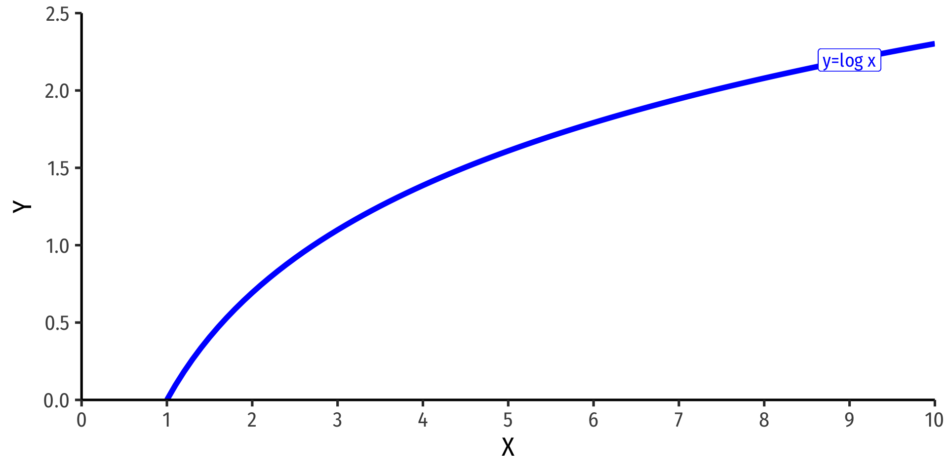
The Natural Logarithm
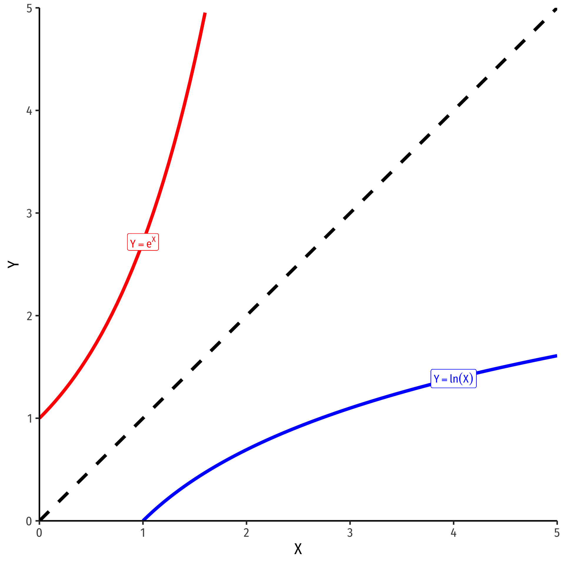
The exponential function, \(Y=e^X\) or \(Y=exp(X)\), where base \(e=2.71828...\)
Natural logarithm is the inverse, \(Y=ln(X)\)
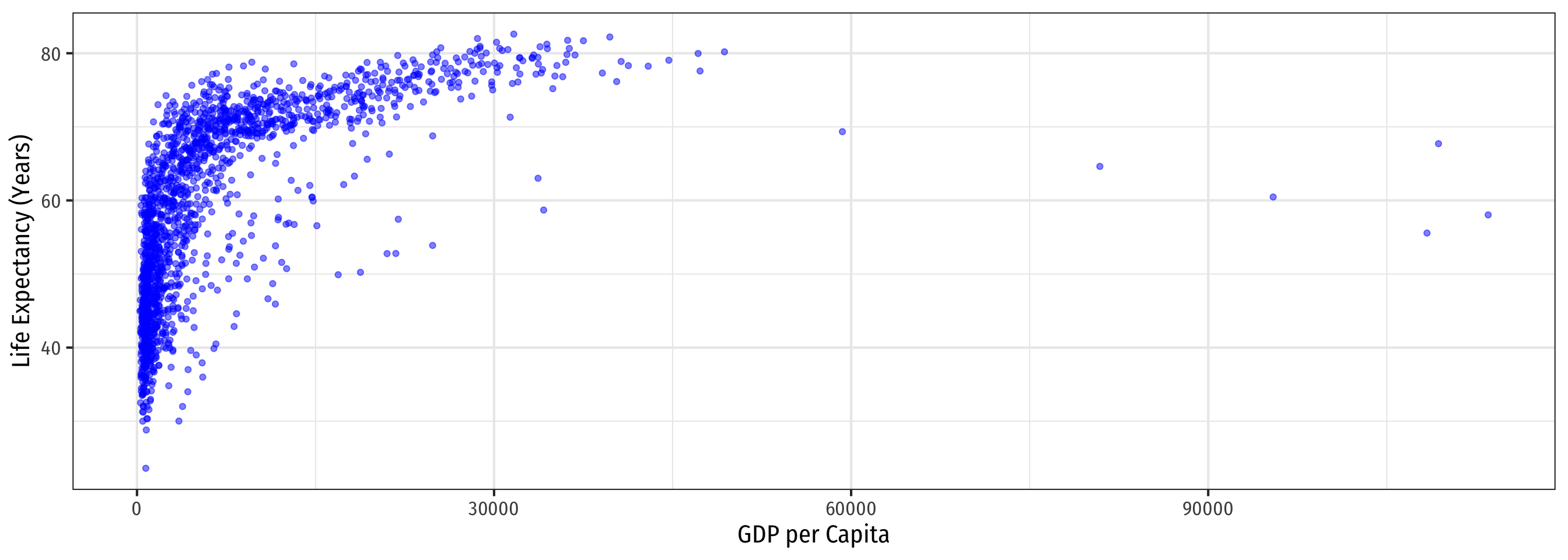
Linear-Log Model Graph (Linear X-Axis)
Code
ggplot(data = gapminder)+
  aes(x = gdpPercap,
      y = lifeExp)+
  geom_point(color = "blue", alpha = 0.5)+
  geom_smooth(method = "lm",
              formula = y ~ log(x),
              color = "orange")+
  scale_x_continuous(labels = scales::dollar,
                     breaks = seq(0,120000,20000))+
  scale_y_continuous(breaks = seq(0,100,10),
                     limits = c(0,100))+
  labs(x = "GDP per Capita",
       y = "Life Expectancy (Years)")+
  theme_bw(base_family = "Fira Sans Condensed",
           base_size = 16)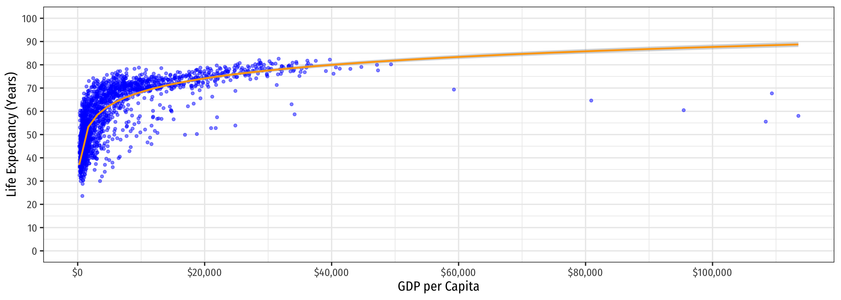
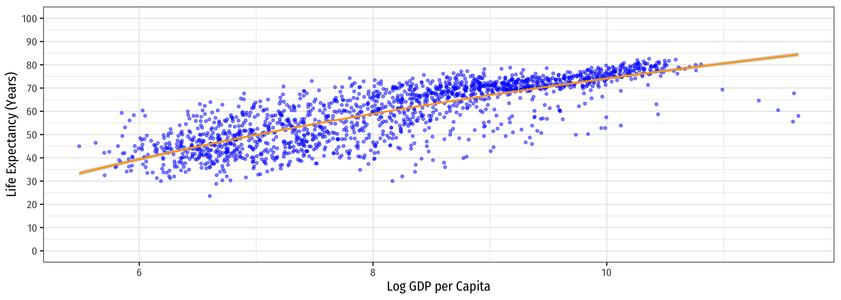
Linear-Log Model Graph (Log X-Axis)
Code
ggplot(data = gapminder)+
  aes(x = loggdp,
      y = lifeExp)+
  geom_point(color = "blue", alpha = 0.5)+
  geom_smooth(method = "lm",
              formula = y ~ log(x),
              color = "orange")+
  scale_y_continuous(breaks = seq(0,100,10),
                     limits = c(0,100))+
  labs(x = "Log GDP per Capita",
       y = "Life Expectancy (Years)")+
  theme_bw(base_family = "Fira Sans Condensed",
           base_size = 16)
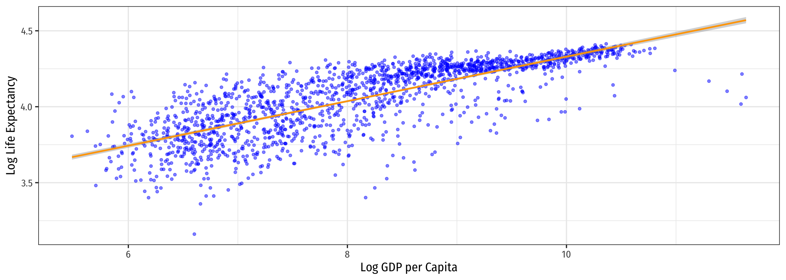
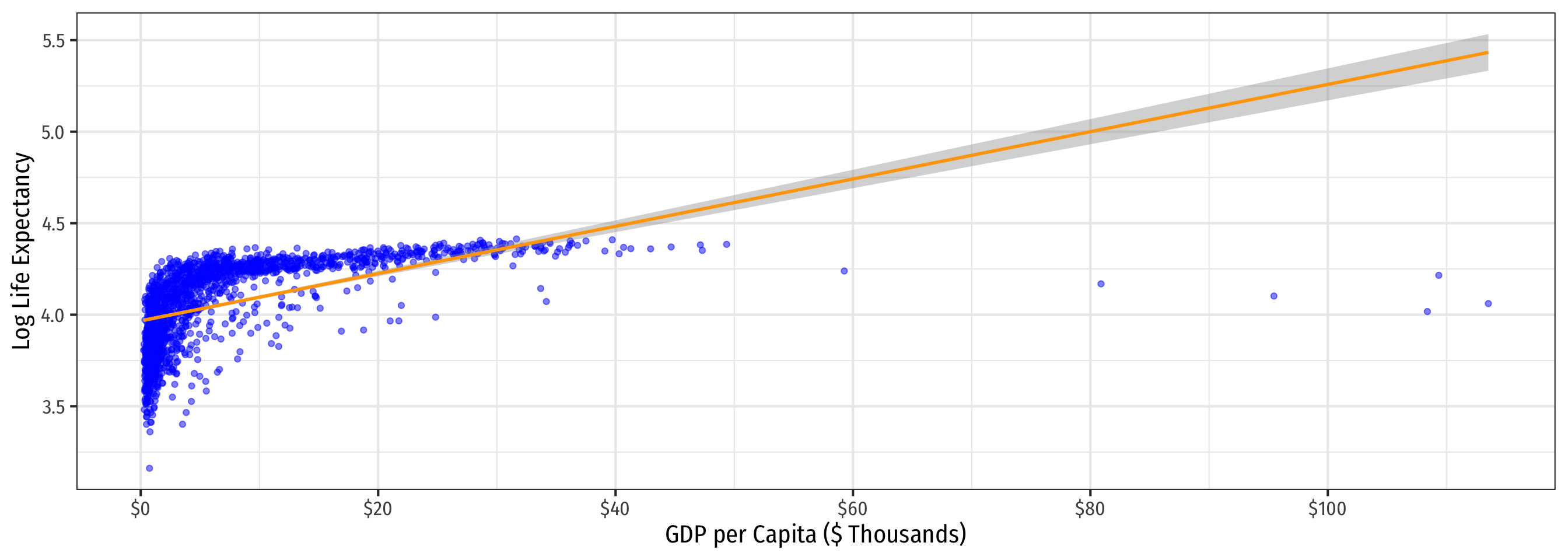
Linear-Log Model Graph
Code
ggplot(data = gapminder)+
  aes(x = gdp_t,
      y = loglife)+
  geom_point(color = "blue", alpha = 0.5)+
  geom_smooth(method = "lm", color = "orange")+
  scale_x_continuous(labels = scales::dollar,
                     breaks = seq(0,120,20))+
  labs(x = "GDP per Capita ($ Thousands)",
       y = "Log Life Expectancy")+
  theme_bw(base_family = "Fira Sans Condensed",
           base_size = 16)
Log-Log Model Graph
Comparing Models III
| Linear-Log | Log-Linear | Log-Log |
|---|---|---|
 |
 |
|
| \(\hat{Y_i}=\hat{\beta_0}+\hat{\beta_1}\color{#e64173}{\ln X_i}\) | \(\color{#e64173}{\ln Y_i}=\hat{\beta_0}+\hat{\beta_1}X_i\) | \(\color{#e64173}{\ln Y_i}=\hat{\beta_0}+\hat{\beta_1}\color{#e64173}{\ln X_i}\) |
| \(R^2=0.65\) | \(R^2=0.30\) | \(R^2=0.61\) |
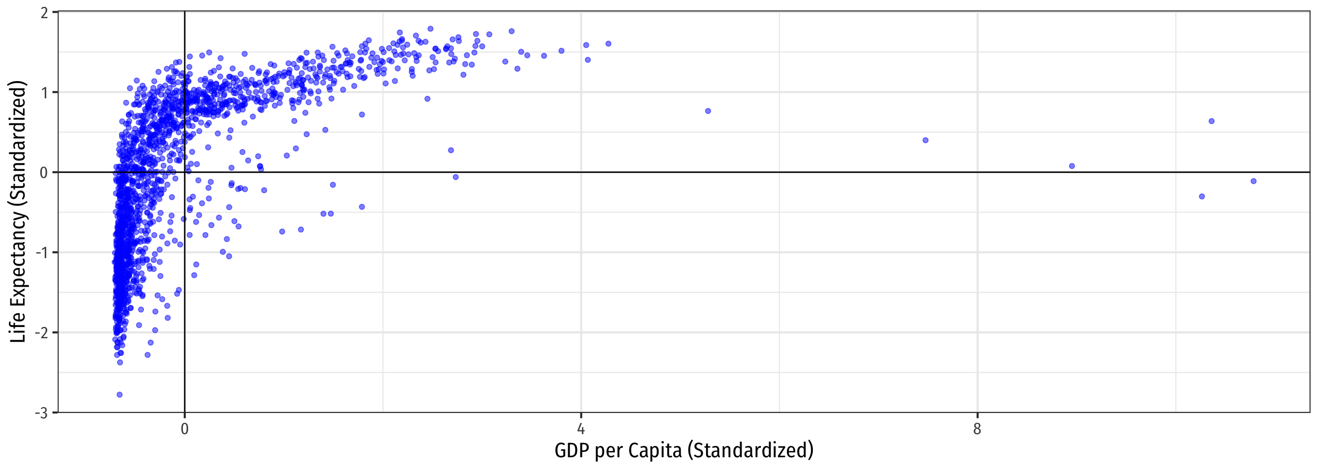
Rescaling: Visually
Rescaling: Visually
All F-test II
- Alternatively, if you use
broominstead ofsummary():glance()command makes table of regression summary statisticstidy()only shows coefficients
statisticis the All F-test,p.valuenext to it is the p-value from the F test
