Types of Data II
- Cross-sectional data: compare different individual \(i\)’s at same time \(\bar{t}\)
\[\hat{Y}_{\color{red}{i}} = \beta_0 + \beta_1 X_{\color{red}{i}} + u_{\color{red}{i}}\]
- Time-series data: track same individual \(\bar{i}\) over different times \(t\)
\[\hat{Y}_{\color{blue}{t}} = \beta_0 + \beta_1 X_{\color{blue}{t}} + u_{\color{blue}{t}}\]
- Panel data: combines these dimensions: compare all individual \(i\)’s over all time \(t\)’s
Panel Data I
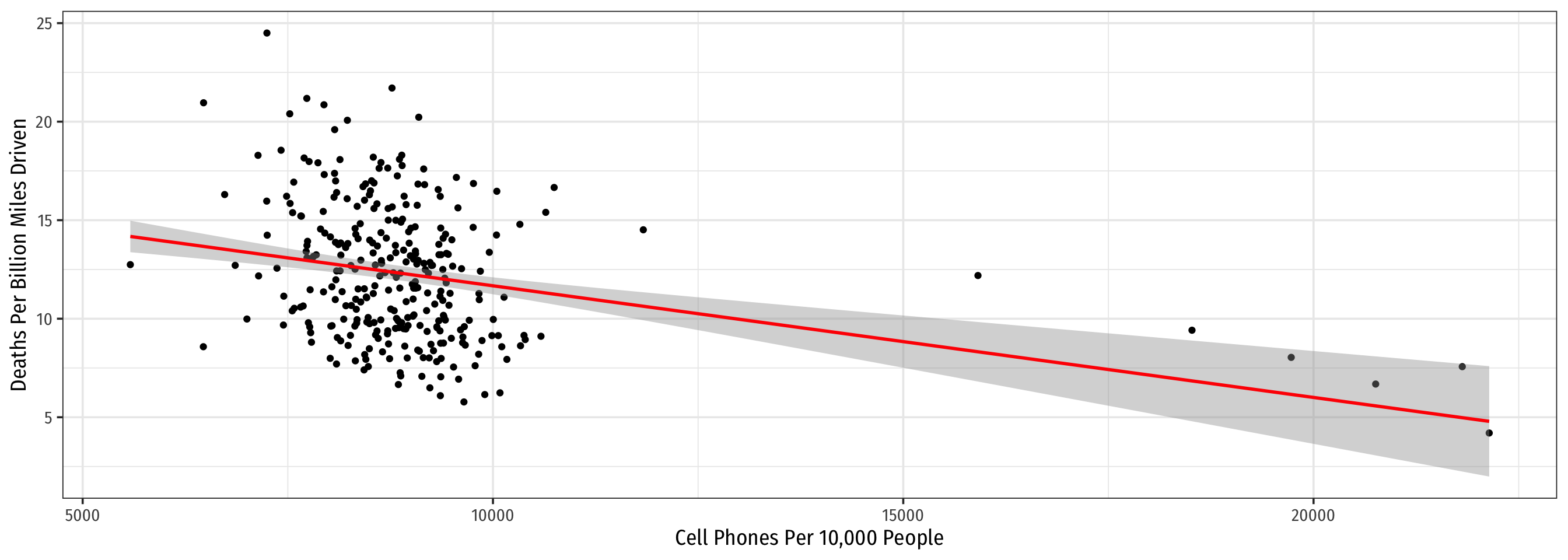
Pooled Regression III
Pooled Regression III
Recall: Assumptions about Errors
- We make 4 critical assumptions about \(u\):
- The expected value of the errors is 0
\[\mathbb{E}[u]=0\]
- The variance of the errors over \(X\) is constant:
\[var(u|X)=\sigma^2_{u}\]
- Errors are not correlated across observations:
\[cor(u_i,u_j)=0 \quad \forall i \neq j\]
- There is no correlation between \(X\) and the error term:
\[cor(X, u)=0 \text{ or } E[u|X]=0\]

Example: Consider Just 5 States
Code
phones %>%
  filter(state %in% c("District of Columbia",
                      "Maryland", "Texas",
                      "California", "Kansas")) %>%
ggplot()+
  aes(x = cell_plans,
      y = deaths,
      color = state)+
  geom_point()+
  geom_smooth(method = "lm")+
  labs(x = "Cell Phones Per 10,000 People",
       y = "Deaths Per Billion Miles Driven",
       color = NULL)+
  theme_bw(base_family = "Fira Sans Condensed",
           base_size = 14)+
  theme(legend.position = "top")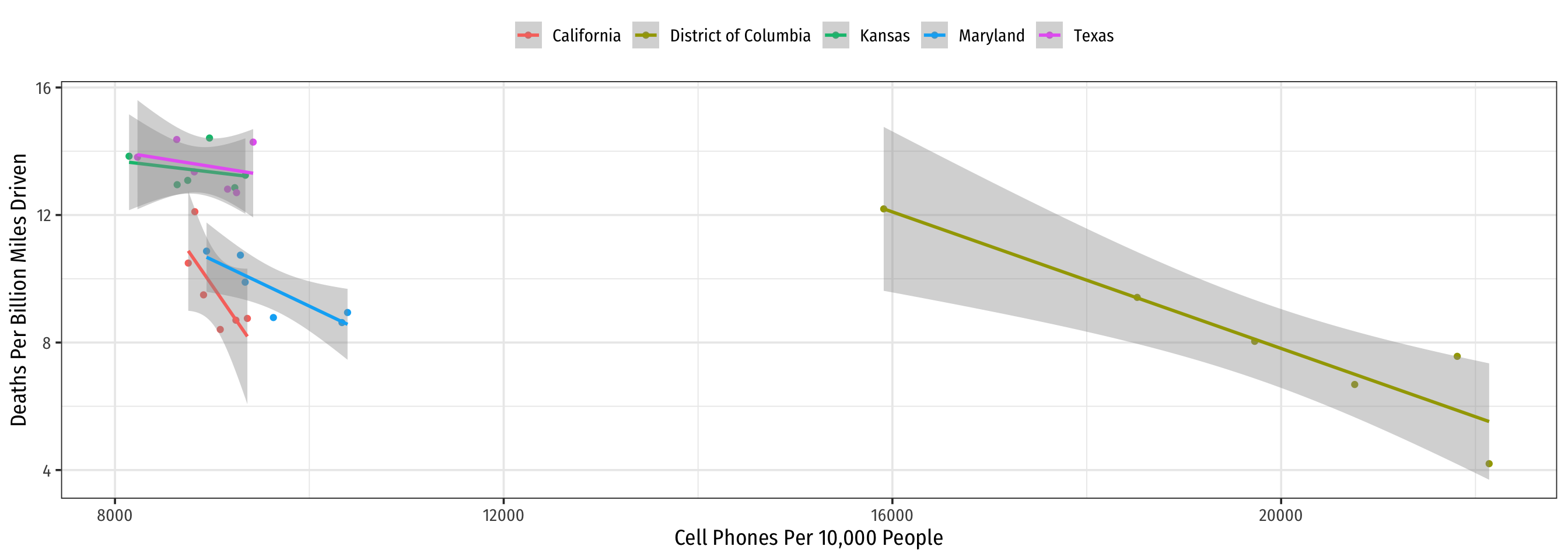
Example: Consider Just 5 States
Code
phones %>%
  filter(state %in% c("District of Columbia",
                      "Maryland", "Texas",
                      "California", "Kansas")) %>%
ggplot()+
  aes(x = cell_plans,
      y = deaths,
      color = state)+
  geom_point()+
  geom_smooth(method = "lm")+
  labs(x = "Cell Phones Per 10,000 People",
       y = "Deaths Per Billion Miles Driven",
       color = NULL)+
  theme_bw(base_family = "Fira Sans Condensed",
           base_size = 14)+
  theme(legend.position = "top")+
  facet_wrap(~state, ncol = 3)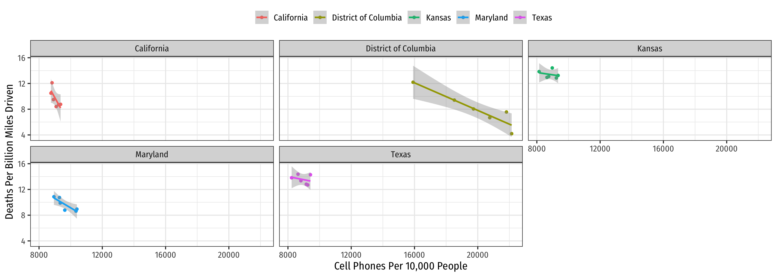
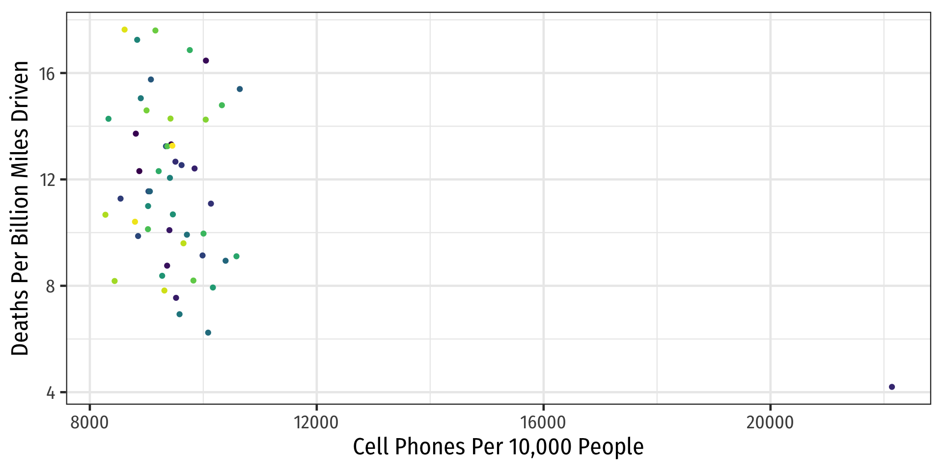
Example: Consider All 51 States
Code
ggplot(data = phones)+
  aes(x = cell_plans,
      y = deaths,
      color = state)+
  geom_point()+
  geom_smooth(method = "lm")+
  labs(x = "Cell Phones Per 10,000 People",
       y = "Deaths Per Billion Miles Driven",
       color = NULL)+
  theme_bw(base_family = "Fira Sans Condensed",
           base_size = 14)+
  theme(legend.position = "none")+
  facet_wrap(~state, ncol = 7)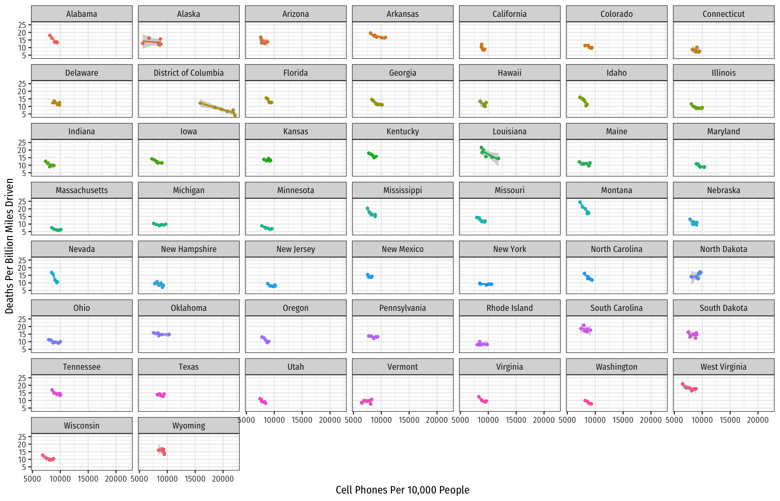
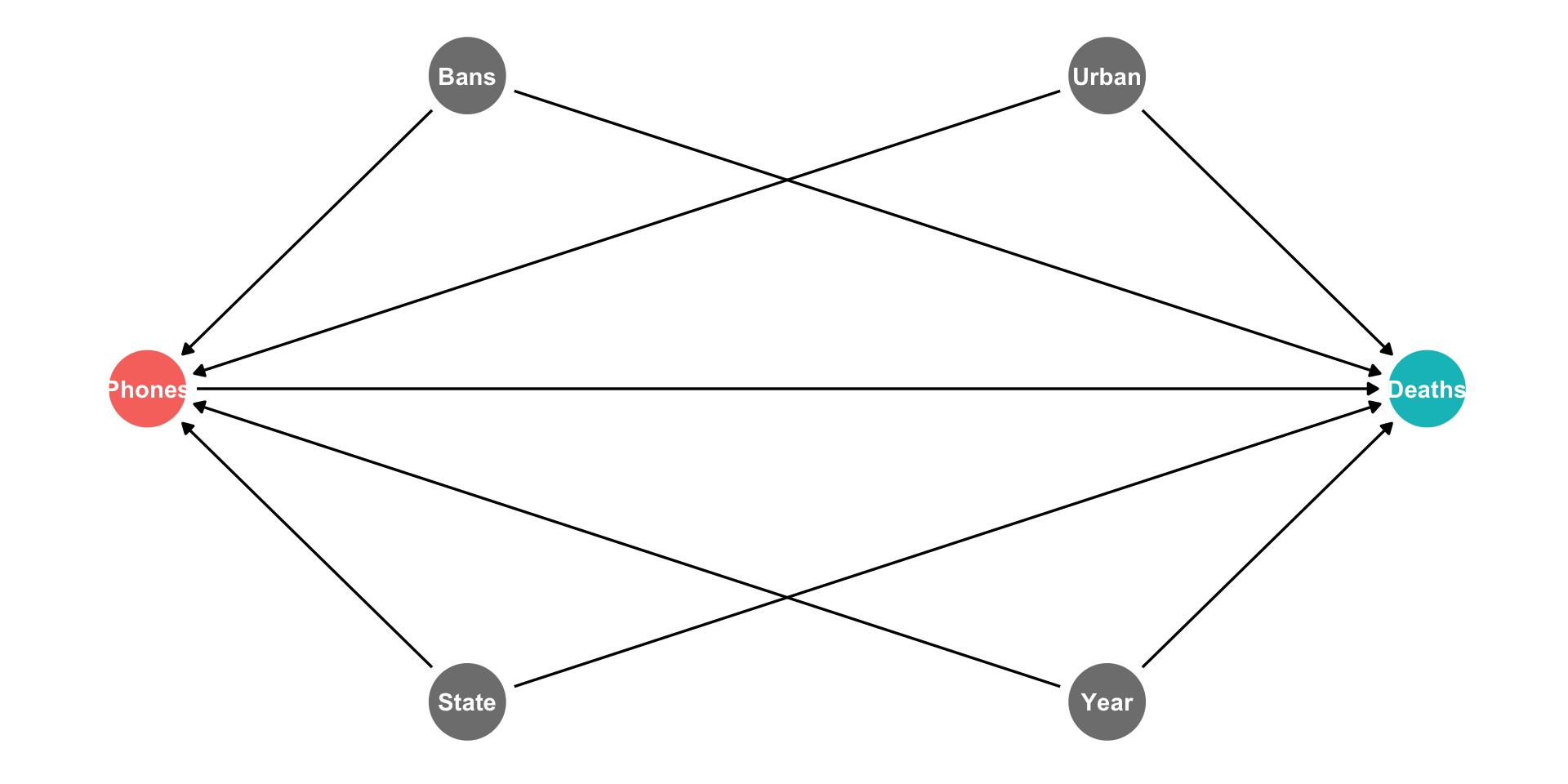
Fixed Effects: DAG I
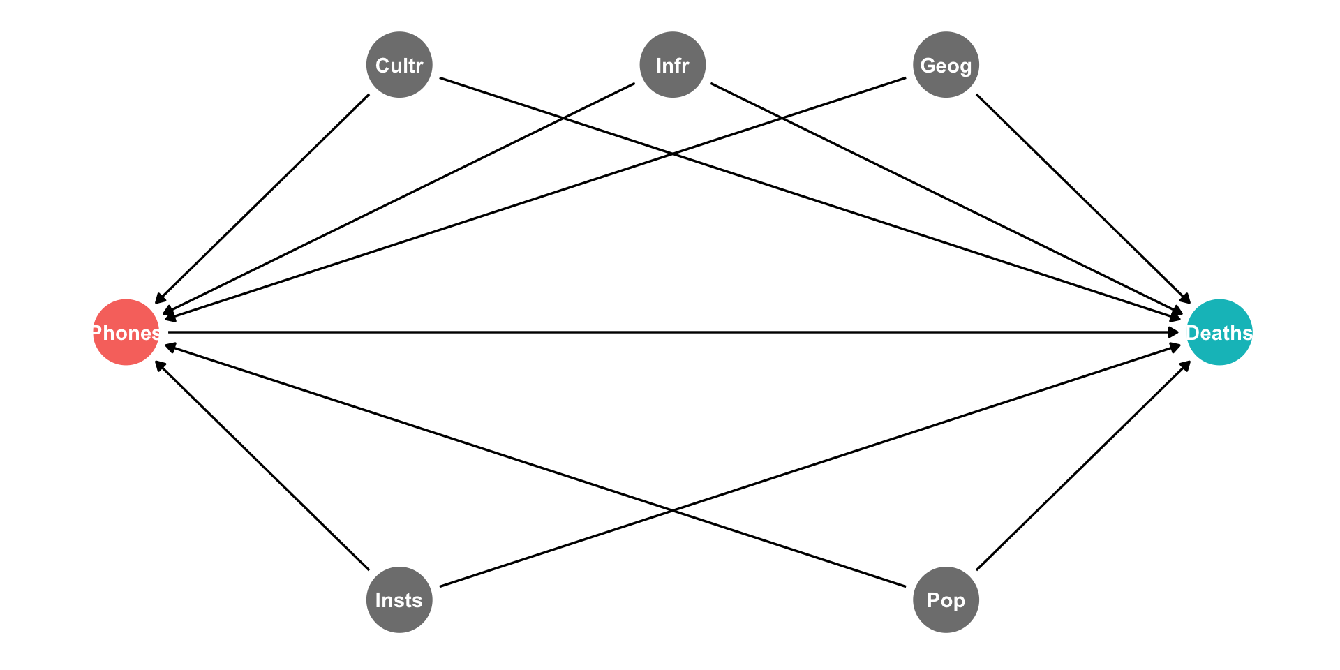
A simple pooled model likely contains lots of omitted variable bias
Many (often unobservable) factors that determine both Phones & Deaths
- Culture, infrastructure, population, geography, institutions, etc
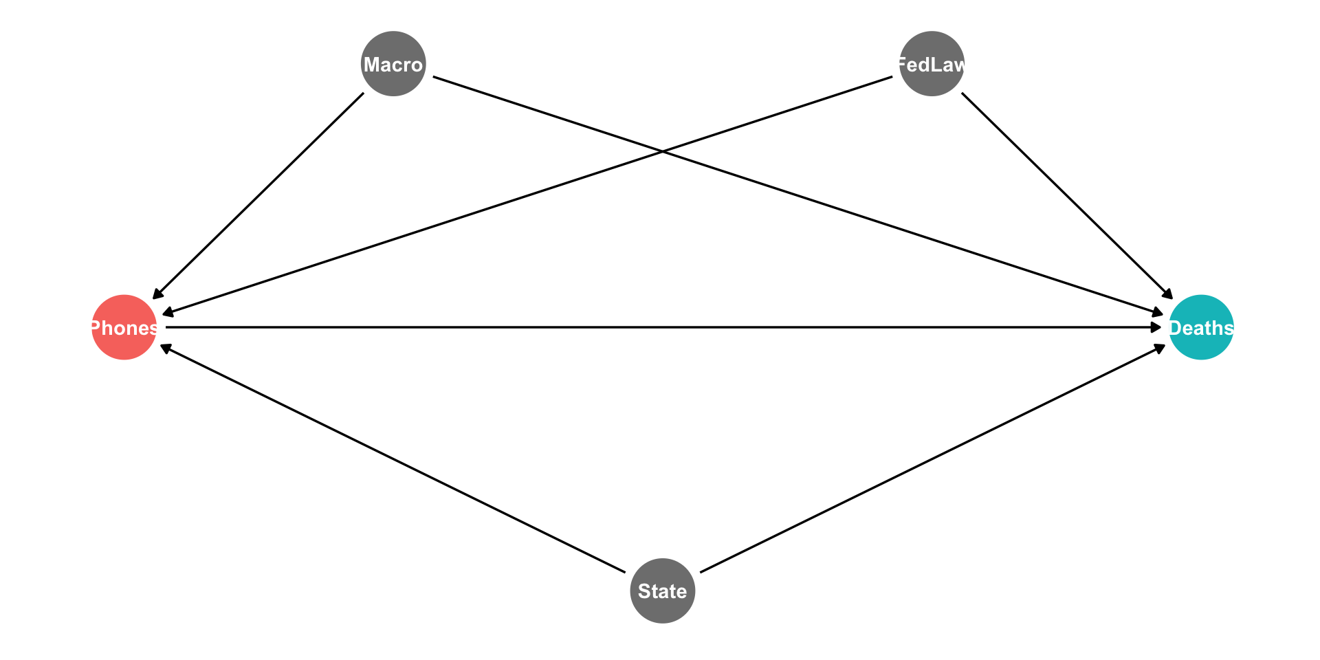
Fixed Effects: DAG II
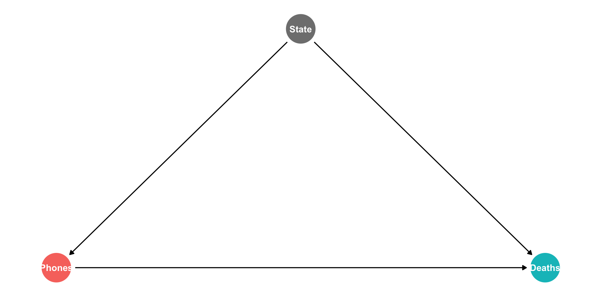
A simple pooled model likely contains lots of omitted variable bias
Many (often unobservable) factors that determine both Phones & Deaths
- Culture, infrastructure, population, geography, institutions, etc
But the beauty of this is that most of these factors systematically vary by U.S. State and are stable over time!
We can simply “control for State” to safely remove the influence of all of these factors!
Looking at the Data in R II
Code
ggplot(data = means_state)+
  aes(x = fct_reorder(state, avg_deaths),
      y = avg_deaths,
      color = state)+
  geom_point()+
  geom_segment(aes(y = 0,
                   yend = avg_deaths,
                   x = state,
                   xend = state))+
  coord_flip()+
  labs(x = "State",
       y = "Deaths Per Billion Miles Driven",
       color = NULL,
       title = "Deaths Vary By State")+
  theme_bw(base_family = "Fira Sans Condensed",
           base_size=10)+
  theme(legend.position = "none")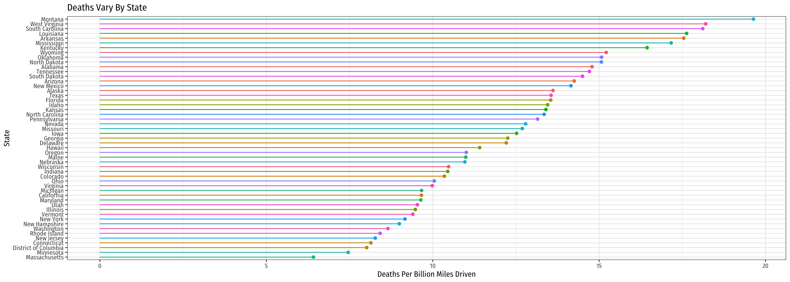
Looking at the Data in R III
Code
ggplot(data = means_state)+
  aes(x = fct_reorder(state, avg_phones),
      y = avg_phones,
      color = state)+
  geom_point()+
  geom_segment(aes(y = 0,
                   yend = avg_phones,
                   x = state,
                   xend = state))+
  coord_flip()+
  labs(x = "State",
       y = "Cell Phone Plans Per 10,000 Population",
       color = NULL,
       title = "Cell Phone Plans Vary By State")+
  theme_bw(base_family = "Fira Sans Condensed",
           base_size=10)+
  theme(legend.position = "none")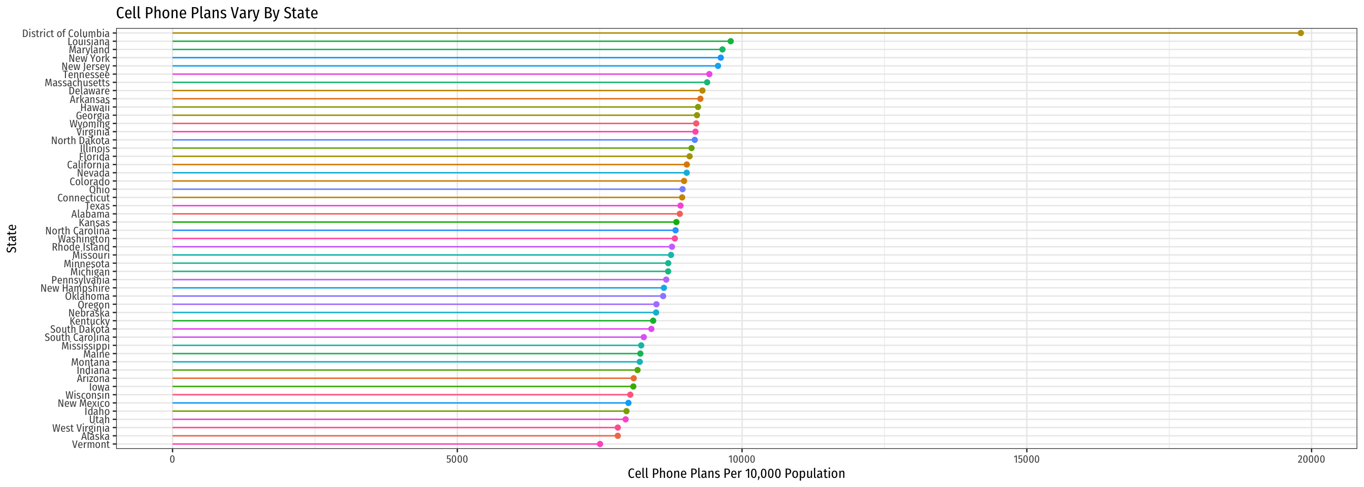
De-Meaning the Data in R: Visualizing
Code
ggplot(data = phones_dm)+
  aes(x = phones_dm,
      y = deaths_dm,
      color = state)+
  geom_point()+
  geom_smooth(method = "lm", color = "black")+
  geom_hline(yintercept = 0)+
  geom_vline(xintercept = 0)+
  labs(x = "De-Meaned Cell Phones Per 10,000 People",
       y = "De-Meaned Deaths Per Billion Miles Driven",
       color = NULL)+
  theme_bw(base_family = "Fira Sans Condensed",
           base_size = 12)+
  theme(legend.position = "none")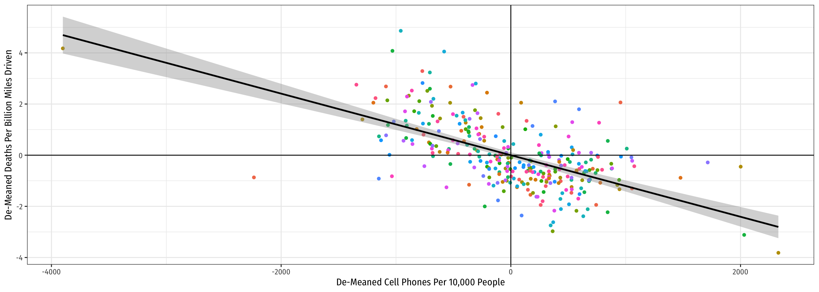
Two-Way Fixed Effects
State fixed effect controls for all factors that vary by state but are stable over time
But there are still other (often unobservable) factors that affect both Phones and Deaths, that don’t vary by State
- The country’s macroeconomic performance, federal laws, etc
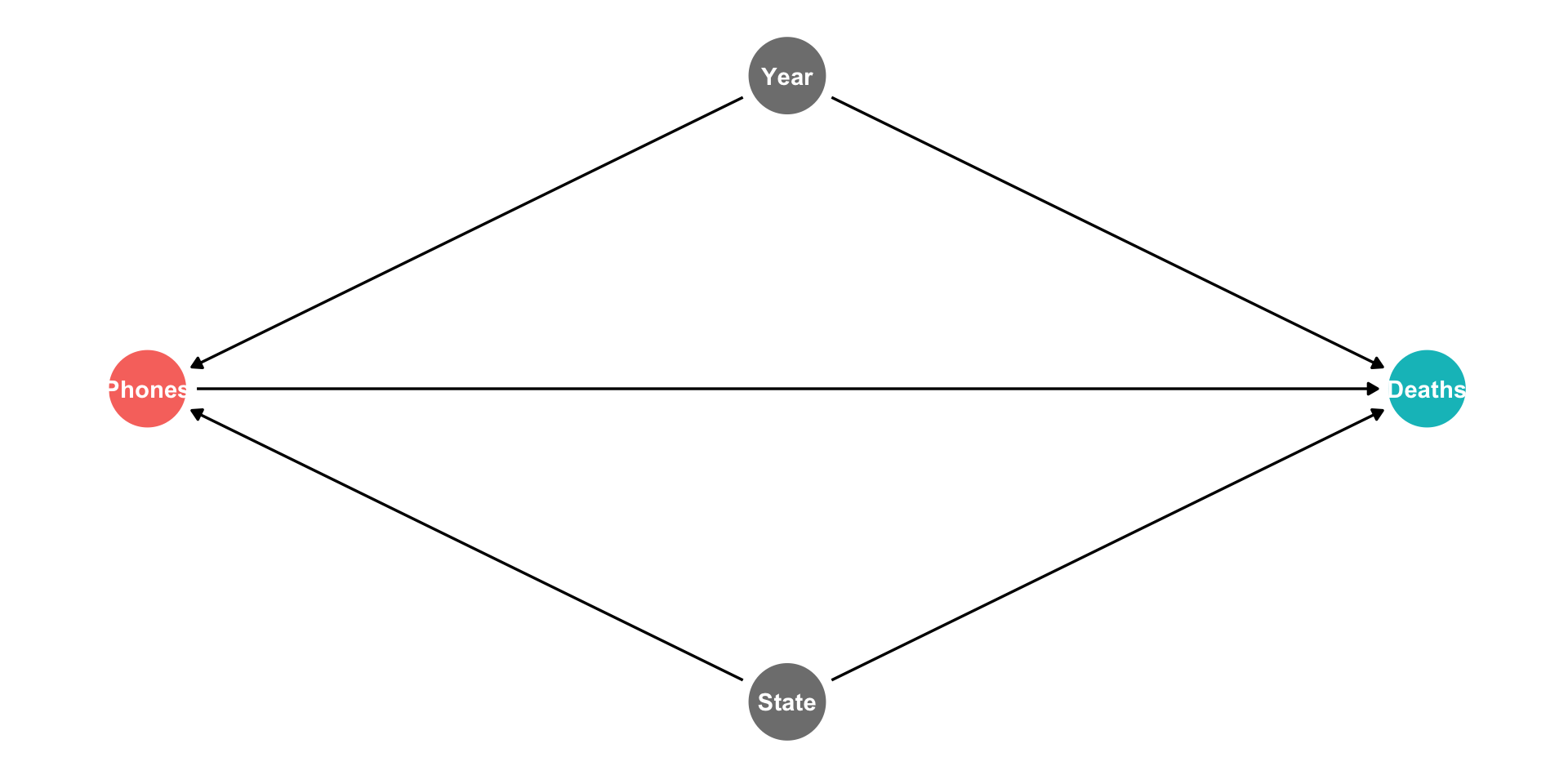
Two-Way Fixed Effects
State fixed effect controls for all factors that vary by state but are stable over time
But there are still other (often unobservable) factors that affect both Phones and Deaths, that don’t vary by State
- The country’s macroeconomic performance, federal laws, etc
If these factors systematically vary over time, but are the same by State, then we can “control for Year” to safely remove the influence of all of these factors!
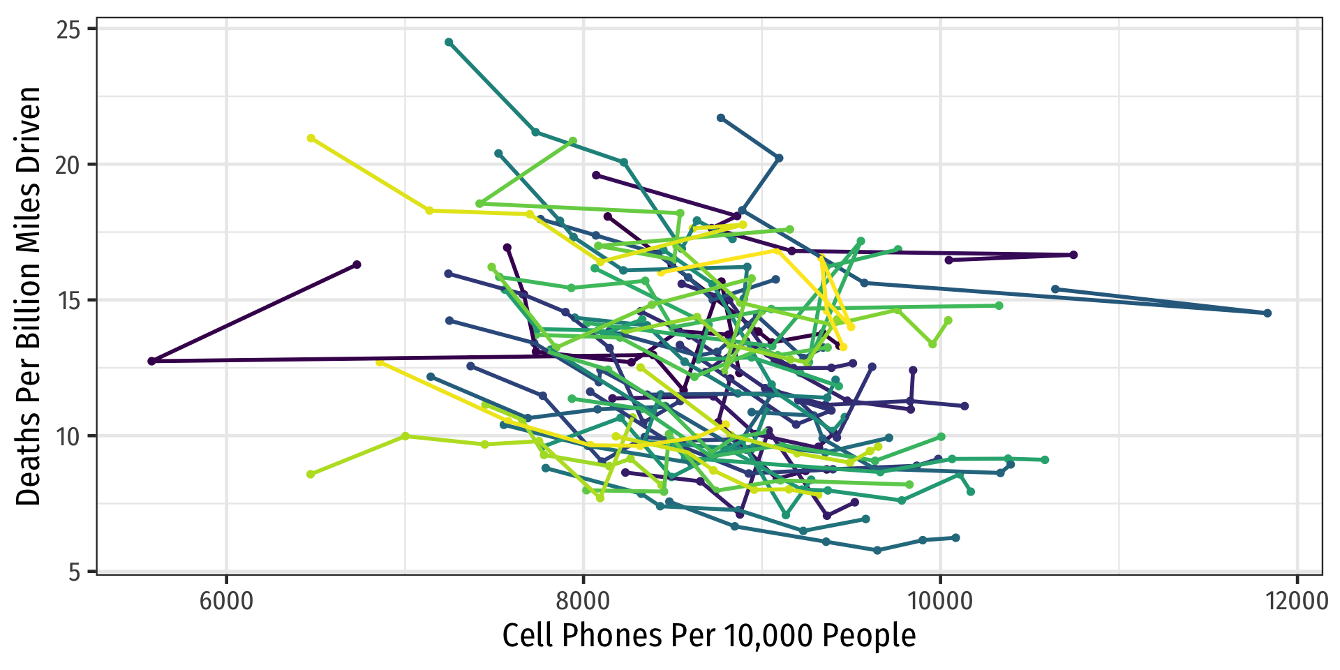
Looking at the Data: Change Over Time
Code
ggplot(data = phones)+
  aes(x = cell_plans,
      y = deaths,
      color = year)+
  geom_point()+
  geom_smooth(method = "lm")+
  labs(x = "Cell Phones Per 10,000 People",
       y = "Deaths Per Billion Miles Driven",
       color = NULL)+
  theme_bw(base_family = "Fira Sans Condensed",
           base_size = 14)+
  theme(legend.position = "none")+
  facet_wrap(~year, ncol = 3)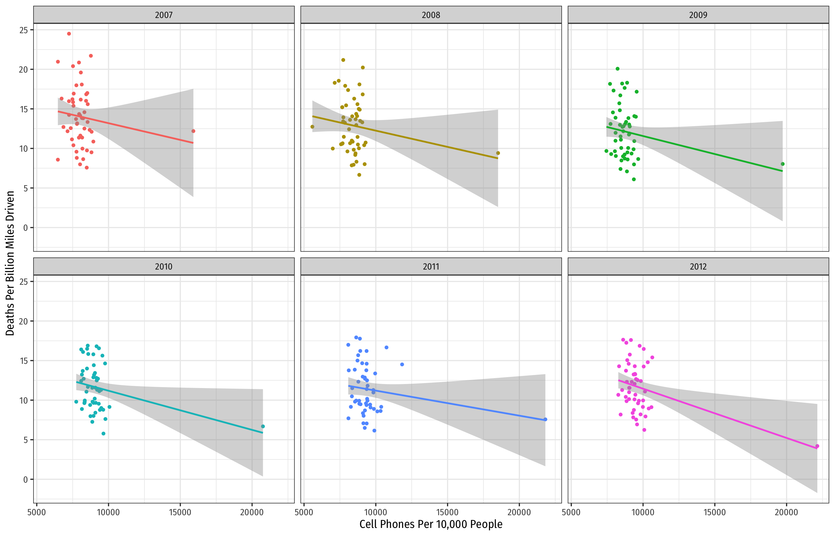
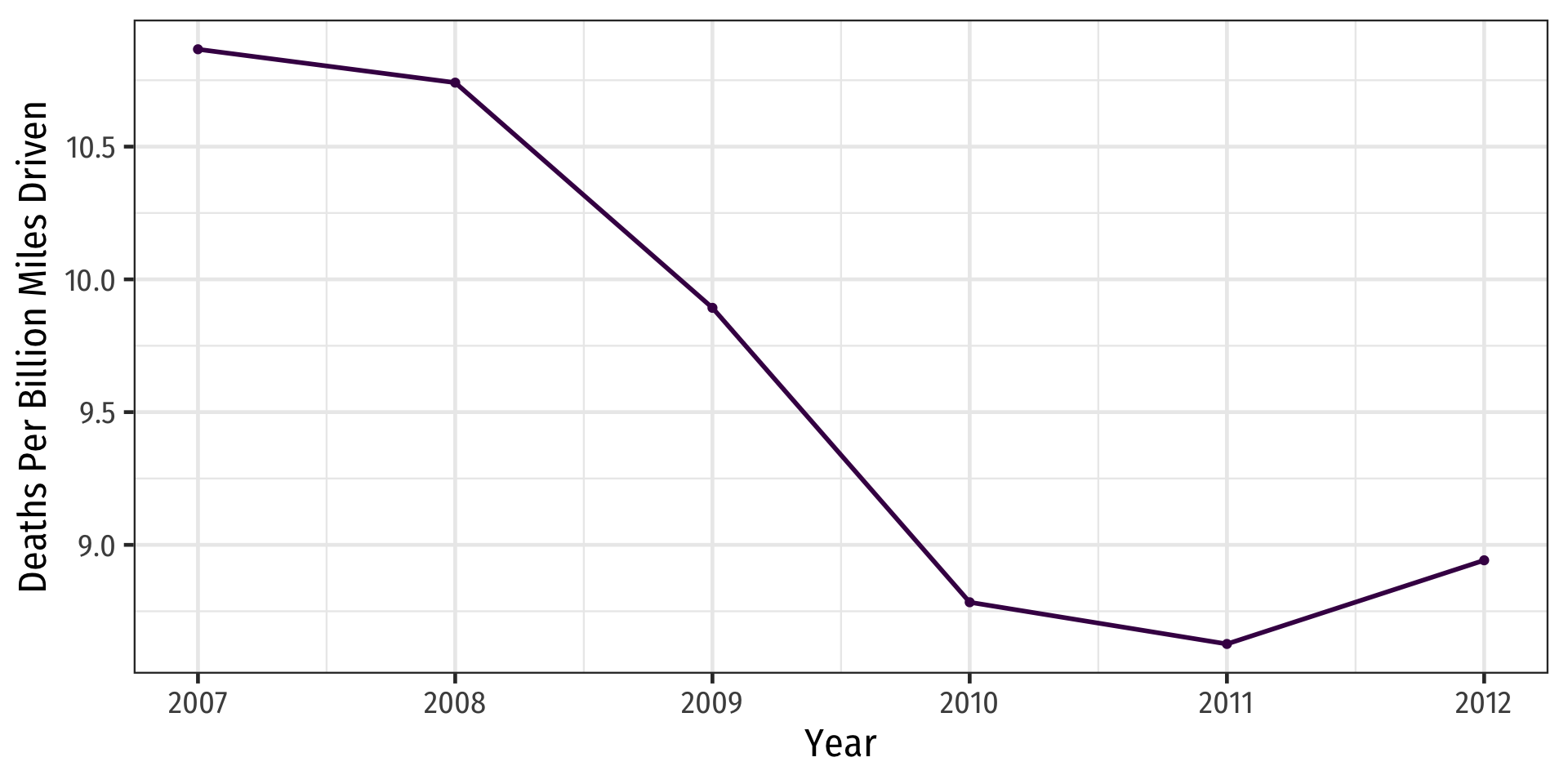
Looking at the Data: Change In Deaths Over Time
Code
ggplot(data = phones)+
  aes(x = year,
      y = deaths)+
  geom_jitter(aes(color = year), width = 0.05)+
  # Add the yearly means as black points
  geom_point(data = means_year,
             aes(x = year,
                 y = avg_deaths),
             size = 3,
             color = "black")+
  # connect the means with a line
  geom_line(data = means_year,
            aes(x = as.numeric(year),
                y = avg_deaths),
            color = "black",
            size = 1)+
  theme_bw(base_family = "Fira Sans Condensed",
           base_size = 14)+
  theme(legend.position = "none")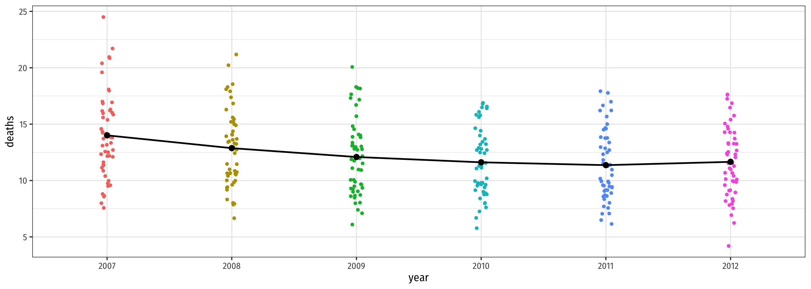
Looking at the Data: Change in Cell Phones Over Time
Code
ggplot(data = phones)+
  aes(x = year,
      y = cell_plans)+
  geom_jitter(aes(color = year), width = 0.05)+
  # Add the yearly means as black points
  geom_point(data = means_year,
             aes(x = year,
                 y = avg_phones),
             size = 3,
             color = "black")+
  # connect the means with a line
  geom_line(data = means_year,
            aes(x = as.numeric(year),
                y = avg_phones),
            color = "black",
            size = 1)+
  theme_bw(base_family = "Fira Sans Condensed",
           base_size = 14)+
  theme(legend.position = "none")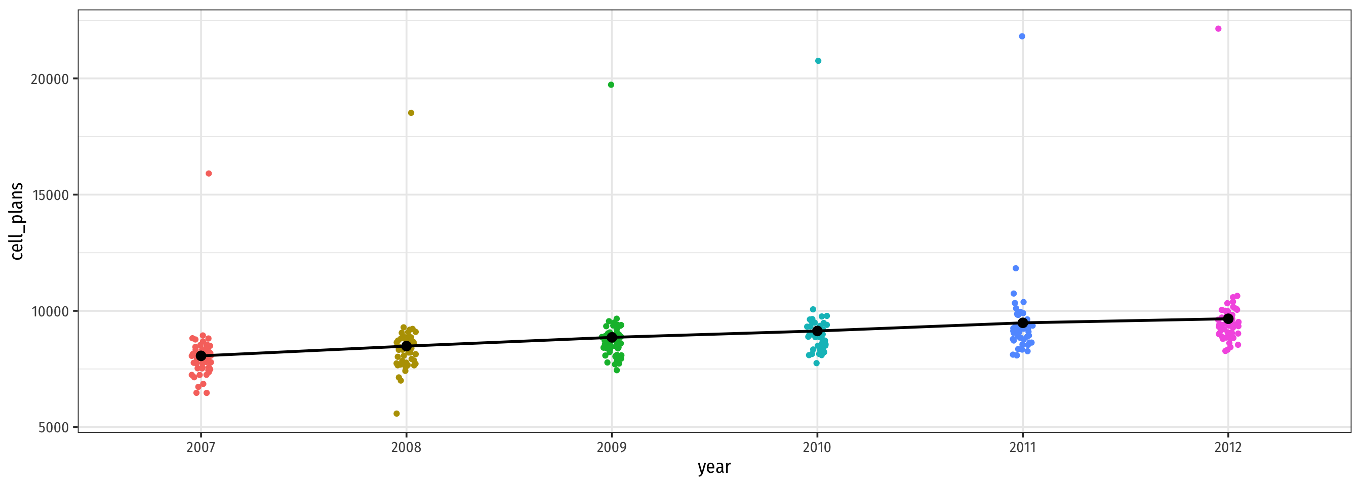
Adding Covariates I
State fixed effect absorbs all unobserved factors that vary by state, but are constant over time
Year fixed effect absorbs all unobserved factors that vary by year, but are constant over States
But there are still other (often unobservable) factors that affect both Phones and Deaths, that vary by State and change over time!
- Some States change their laws during the time period
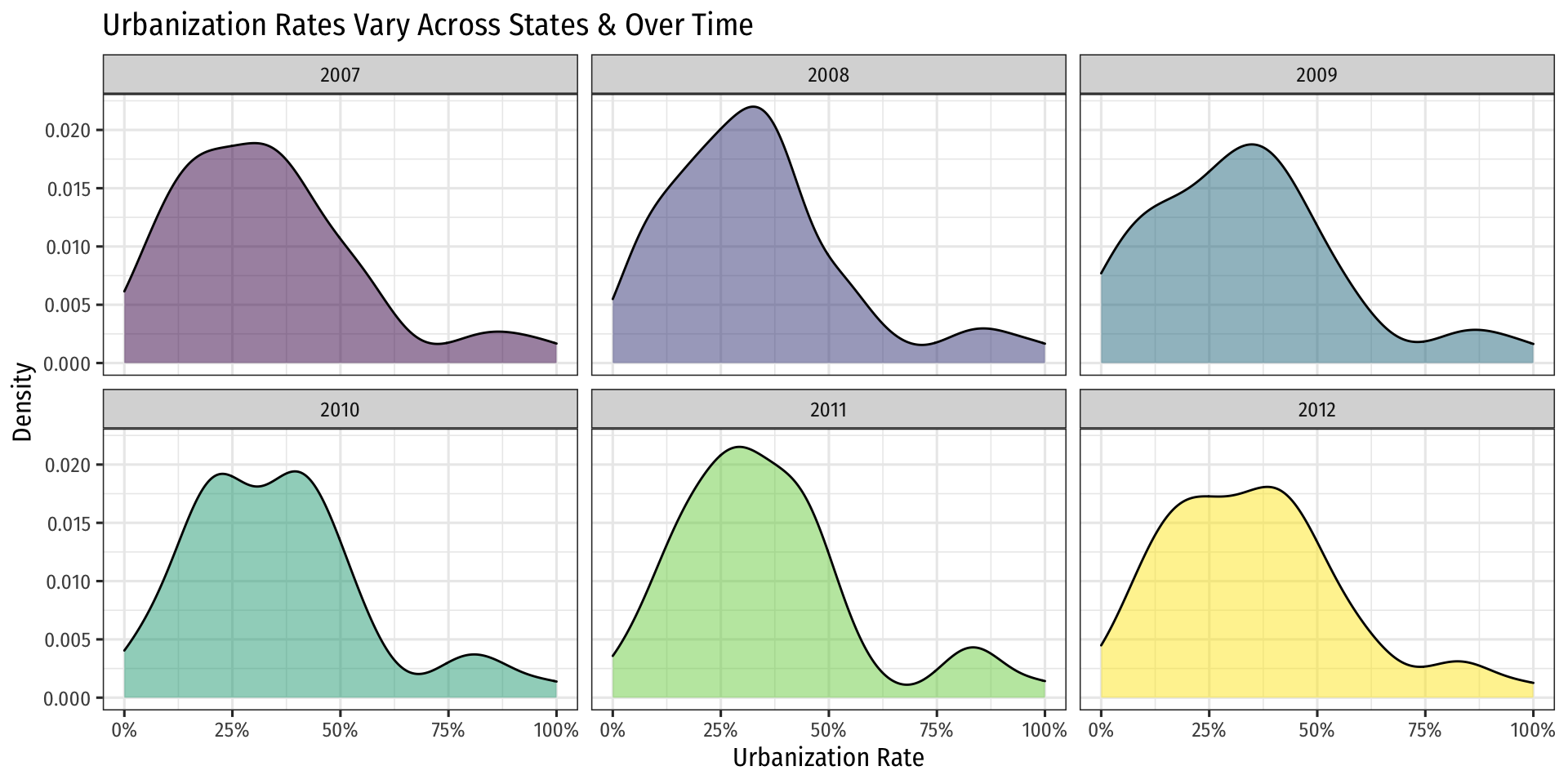
- State urbanization rates change over the time period
We will also need to control for these variables (not picked up by fixed effects!)
- Add them to the regression
Adding Covariates — Necessary?
Comparing Models
| Pooled Regression | State FE | State & Year FE | TWFE with Controls | |
|---|---|---|---|---|
| Constant | 17.33710*** | |||
| (0.97538) | ||||
| Cell Phone Plans | −0.00057*** | −0.00120*** | −3e−04 | −0.00034 |
| (0.00011) | (0.00014) | (0.00031) | (0.00028) | |
| text_ban1 | 0.25593 | |||
| (0.24344) | ||||
| urban_percent | 0.01313 | |||
| (0.00982) | ||||
| cell_ban1 | −0.67980** | |||
| (0.33566) | ||||
| n | 306 | 306 | 306 | 306 |
| Adj. R2 | 0.08 | |||
| SER | 3.27 | 1.05 | 0.93 | 0.92 |
| * p < 0.1, ** p < 0.05, *** p < 0.01 |
