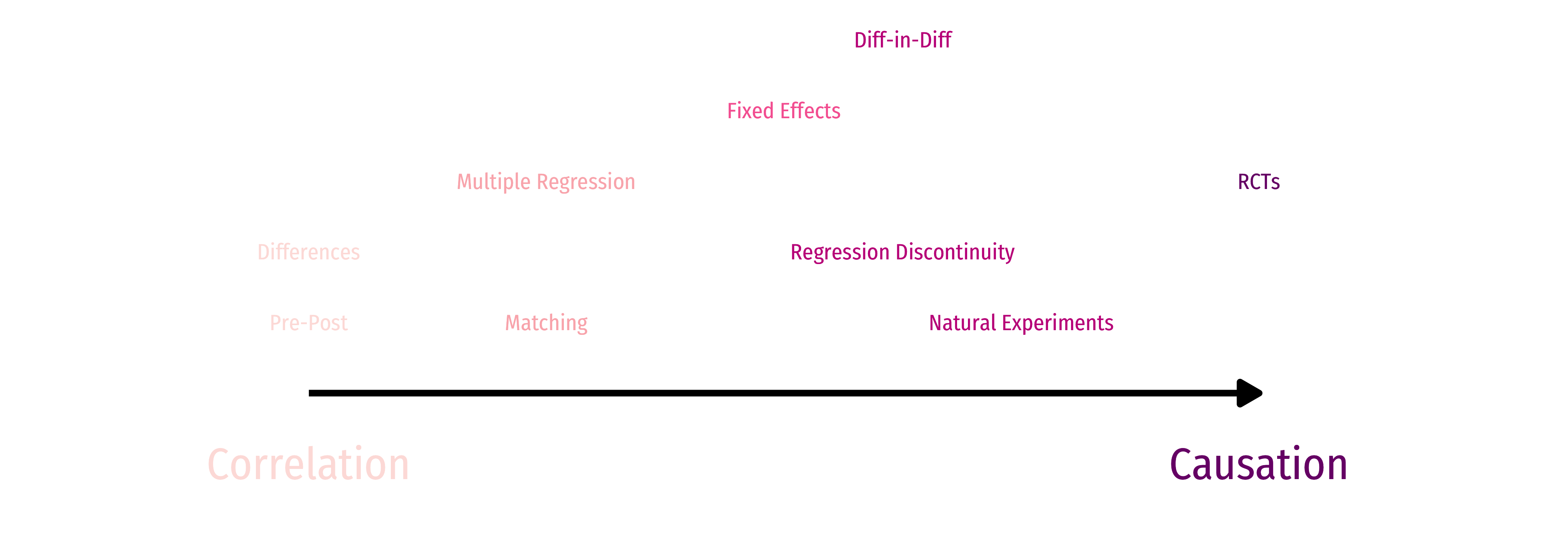
Clever Research Designs Identify Causality
Again, this toolkit of research designs to identify causal effects is the economist’s comparative advantage that firms and governments want!
Natural Experiments

Difference-in-Differences Models I
- Often, we want to examine the consequences of a change, such as a law or policy intervention
Example
- How do States that implement policy \(X\) see changes in \(Y\)
- Treatment: States that implement \(X\)
- Control: States that did not implement \(X\)
If we have panel data with observations for all states before and after the change…
Find the difference between treatment & control groups in their differences before and after the treatment period

Example: Hot Dogs

- Is there a discount when you get cheese and chili?
Example: Hot Dogs
- Diff-n-diff is just a model with an interaction term between two dummies!
Visualizing Diff-in-Diff
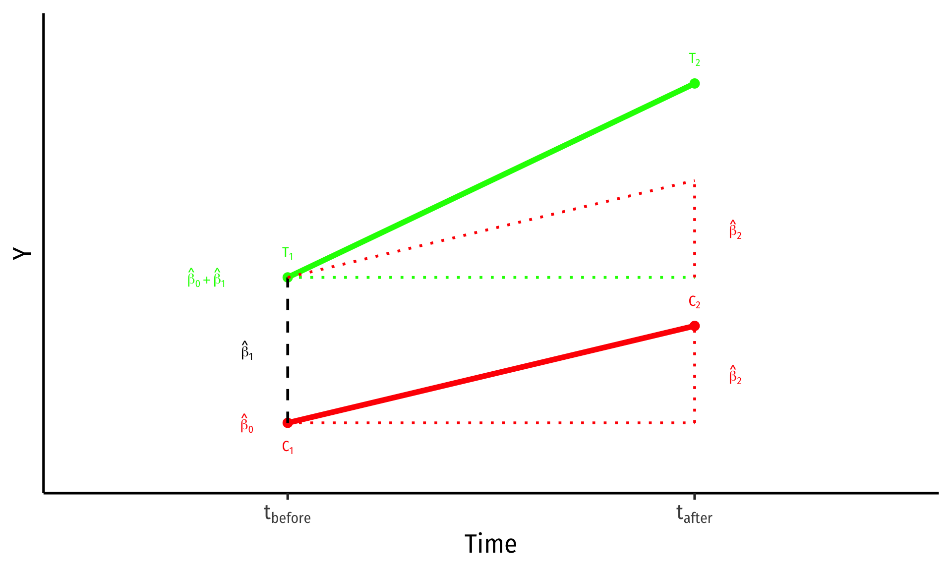
\[\hat{Y}_{it}=\beta_0+\beta_1 \, \text{Treated}_i +\beta_2 \, \text{After}_{t}+\beta_3 \,(\text{Treated}_i \times \text{After}_{t})+u_{it}\]
Control group \((\text{Treated}_i = 0)\)
\(\hat{\beta_0}\): value of \(Y\) for control group before treatment
\(\hat{\beta_2}\): time difference (for control group)
Visualizing Diff-in-Diff
\[\hat{Y}_{it}=\beta_0+\beta_1 \, \text{Treated}_i +\beta_2 \, \text{After}_{t}+\beta_3 \,(\text{Treated}_i \times \text{After}_{t})+u_{it}\]
Control group \((\text{Treated}_i = 0)\)
\(\hat{\beta_0}\): value of \(Y\) for control group before treatment
\(\hat{\beta_2}\): time difference (for control group)
Treatment group \((\text{Treated}_i = 1)\)
\(\hat{\beta_1}\): difference between groups before treatment
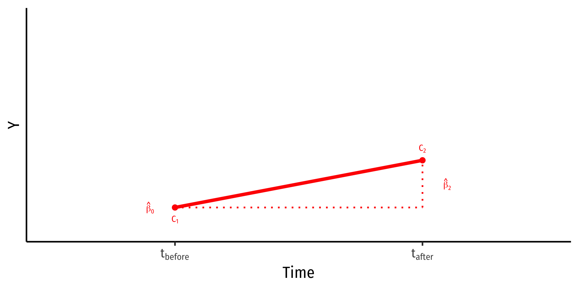
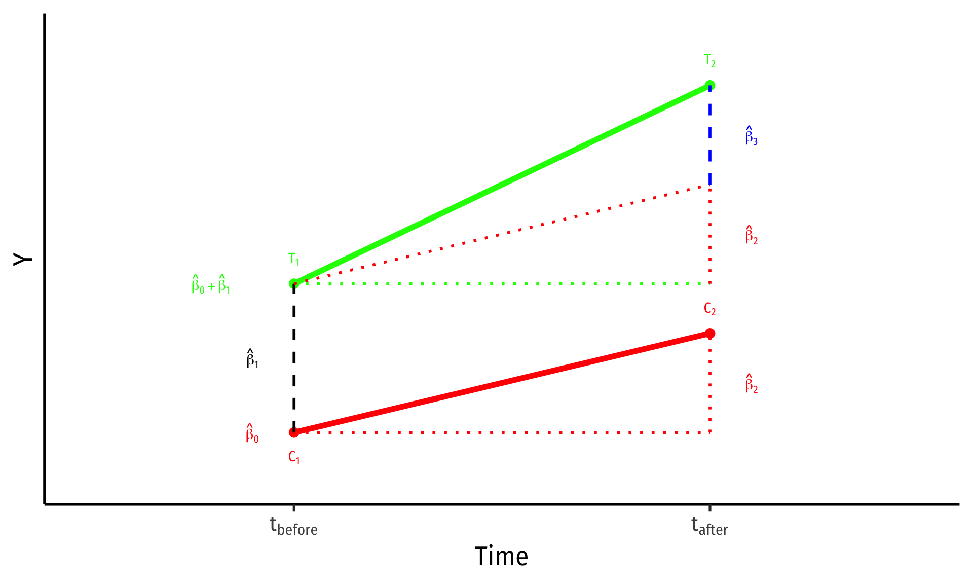
\(\hat{\beta_3}\): difference-in-differences (treatment effect)
Visualizing Diff-in-Diff II
\[\hat{Y}_{it}=\beta_0+\beta_1 \, \text{Treated}_i +\beta_2 \, \text{After}_{t}+\beta_3 \,(\text{Treated}_i \times \text{After}_{t})+u_{it}\]
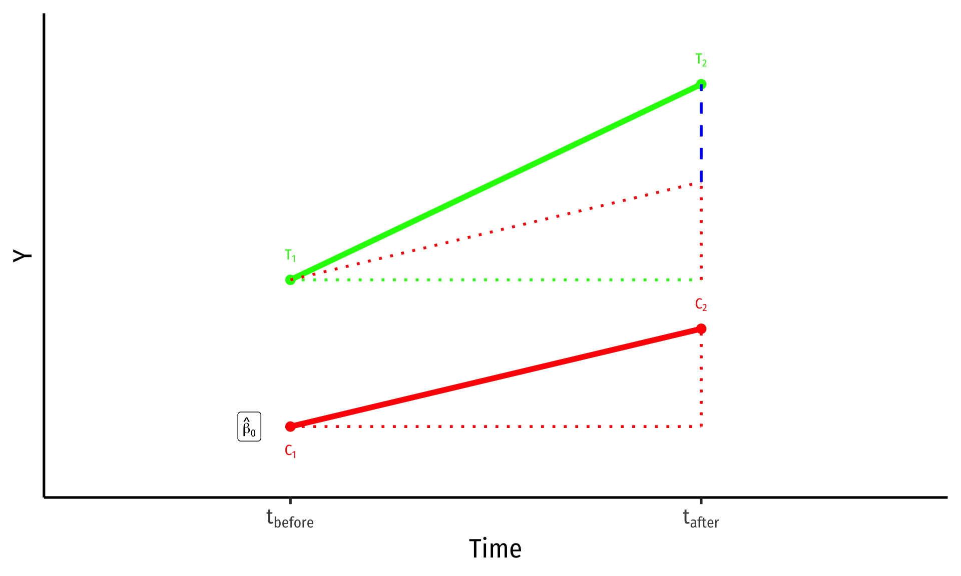
- \(\bar{Y_i}\) for Control group before: \(\hat{\beta_0}\)
Visualizing Diff-in-Diff II
\[\hat{Y}_{it}=\beta_0+\beta_1 \, \text{Treated}_i +\beta_2 \, \text{After}_{t}+\beta_3 \,(\text{Treated}_i \times \text{After}_{t})+u_{it}\]
\(\bar{Y_i}\) for Control group before: \(\hat{\beta_0}\)
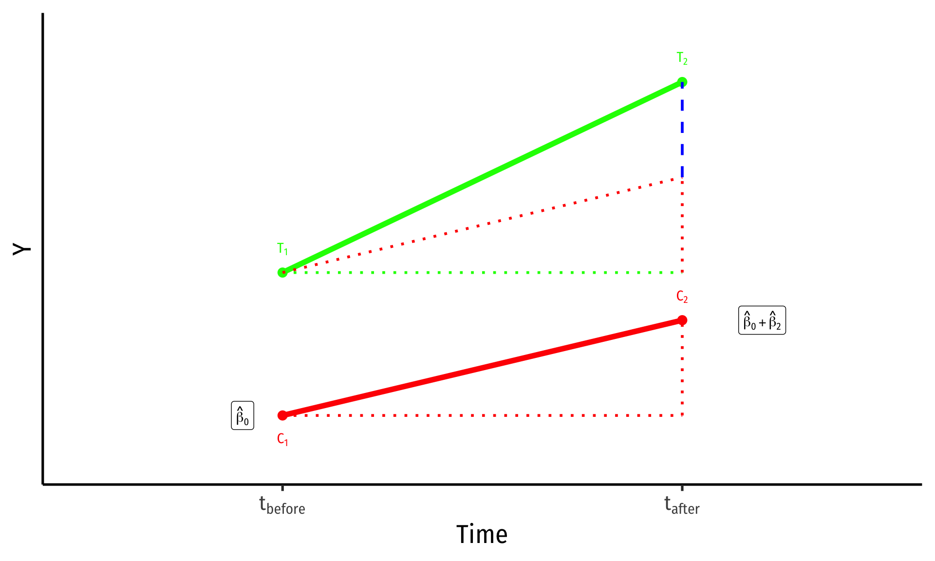
\(\bar{Y_i}\) for Control group after: \(\hat{\beta_0}+\hat{\beta_2}\)
Visualizing Diff-in-Diff II
\[\hat{Y}_{it}=\beta_0+\beta_1 \, \text{Treated}_i +\beta_2 \, \text{After}_{t}+\beta_3 \,(\text{Treated}_i \times \text{After}_{t})+u_{it}\]
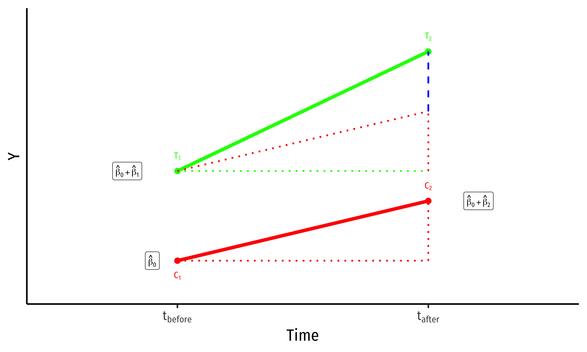
\(\bar{Y_i}\) for Control group before: \(\hat{\beta_0}\)
\(\bar{Y_i}\) for Control group after: \(\hat{\beta_0}+\hat{\beta_2}\)
\(\bar{Y_i}\) for Treatment group before: \(\hat{\beta_0}+\hat{\beta_1}\)
Visualizing Diff-in-Diff II
\[\hat{Y}_{it}=\beta_0+\beta_1 \, \text{Treated}_i +\beta_2 \, \text{After}_{t}+\beta_3 \,(\text{Treated}_i \times \text{After}_{t})+u_{it}\]
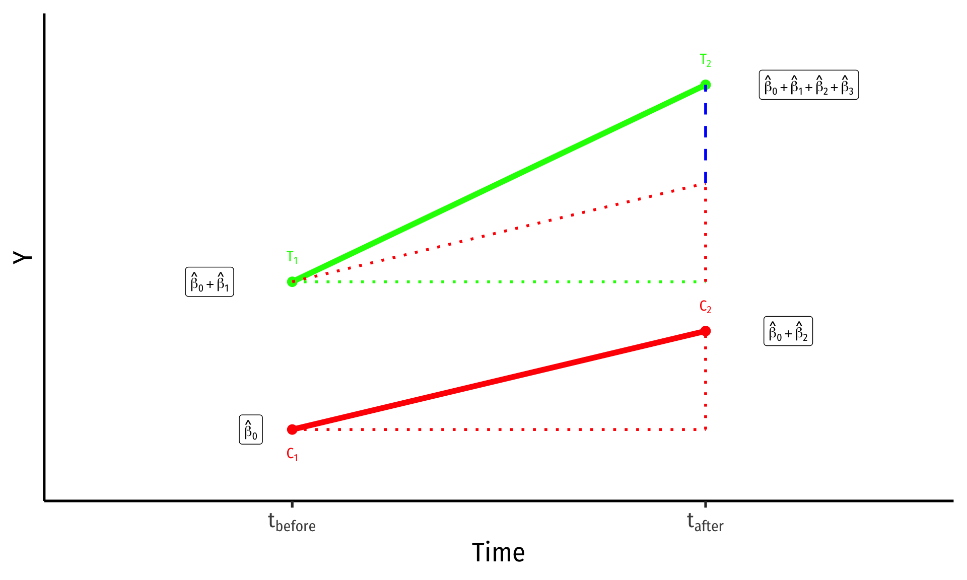
\(\bar{Y_i}\) for Control group before: \(\hat{\beta_0}\)
\(\bar{Y_i}\) for Control group after: \(\hat{\beta_0}+\hat{\beta_2}\)
\(\bar{Y_i}\) for Treatment group before: \(\hat{\beta_0}+\hat{\beta_1}\)
\(\bar{Y_i}\) for Treatment group after: \(\hat{\beta_0}+\hat{\beta_1}+\hat{\beta_2}+\hat{\beta_3}\)
Visualizing Diff-in-Diff II
\[\hat{Y}_{it}=\beta_0+\beta_1 \, \text{Treated}_i +\beta_2 \, \text{After}_{t}+\beta_3 \,(\text{Treated}_i \times \text{After}_{t})+u_{it}\]
\(\bar{Y_i}\) for Control group before: \(\hat{\beta_0}\)
\(\bar{Y_i}\) for Control group after: \(\hat{\beta_0}+\hat{\beta_2}\)
\(\bar{Y_i}\) for Treatment group before: \(\hat{\beta_0}+\hat{\beta_1}\)
\(\bar{Y_i}\) for Treatment group after: \(\hat{\beta_0}+\hat{\beta_1}+\hat{\beta_2}+\hat{\beta_3}\)
Group Difference (before): \(\hat{\beta_1}\)
Visualizing Diff-in-Diff II
\[\hat{Y}_{it}=\beta_0+\beta_1 \, \text{Treated}_i +\beta_2 \, \text{After}_{t}+\beta_3 \,(\text{Treated}_i \times \text{After}_{t})+u_{it}\]
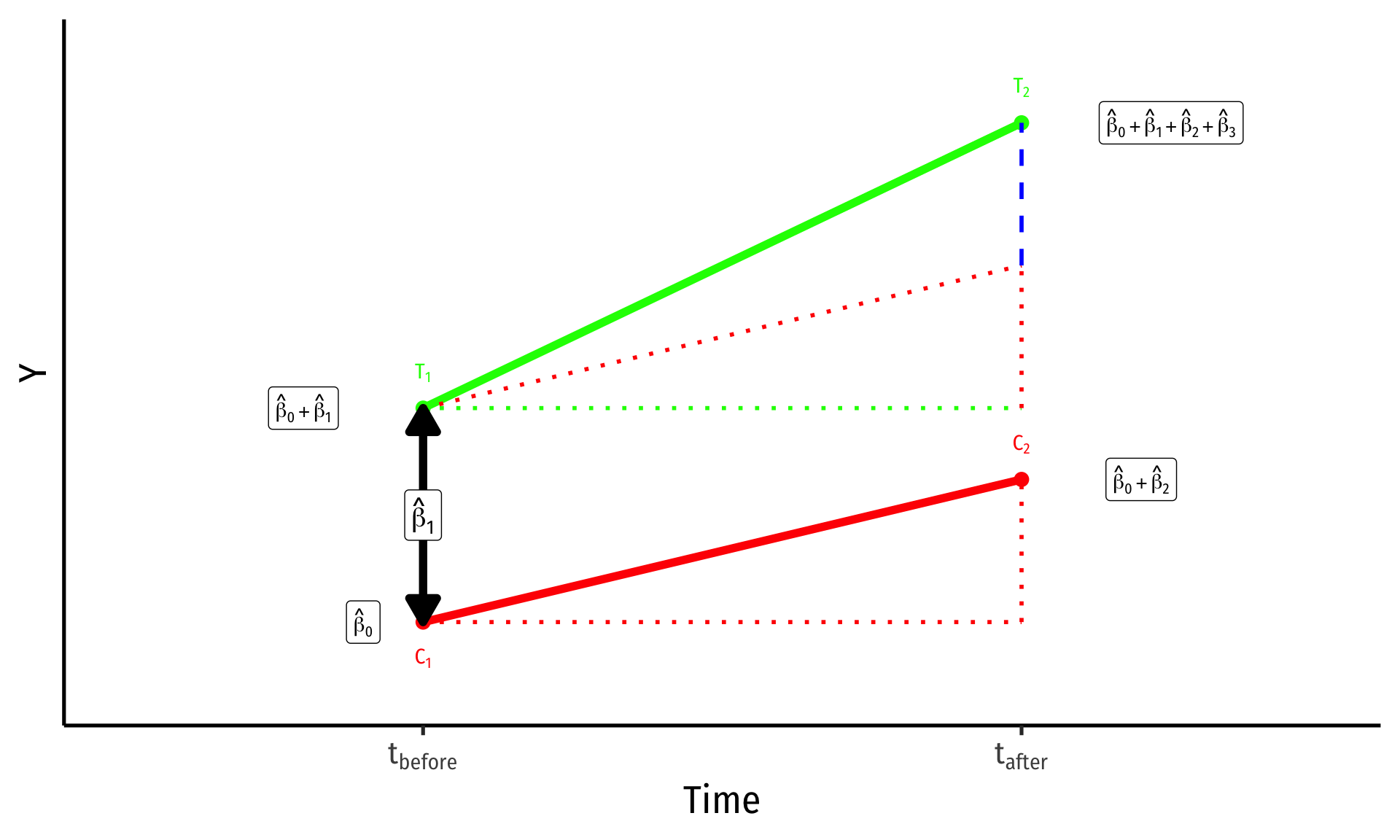
\(\bar{Y_i}\) for Control group before: \(\hat{\beta_0}\)
\(\bar{Y_i}\) for Control group after: \(\hat{\beta_0}+\hat{\beta_2}\)
\(\bar{Y_i}\) for Treatment group before: \(\hat{\beta_0}+\hat{\beta_1}\)
\(\bar{Y_i}\) for Treatment group after: \(\hat{\beta_0}+\hat{\beta_1}+\hat{\beta_2}+\hat{\beta_3}\)
Group Difference (before): \(\hat{\beta_1}\)
Time Difference: \(\hat{\beta_2}\)
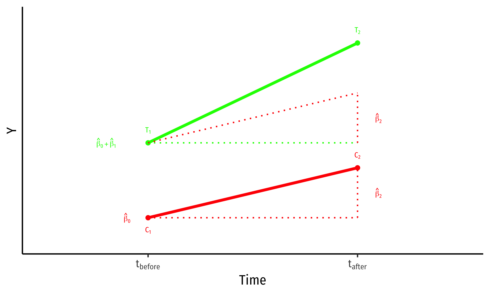
Visualizing Diff-in-Diff II
\[\hat{Y}_{it}=\beta_0+\beta_1 \, \text{Treated}_i +\beta_2 \, \text{After}_{t}+\beta_3 \,(\text{Treated}_i \times \text{After}_{t})+u_{it}\]
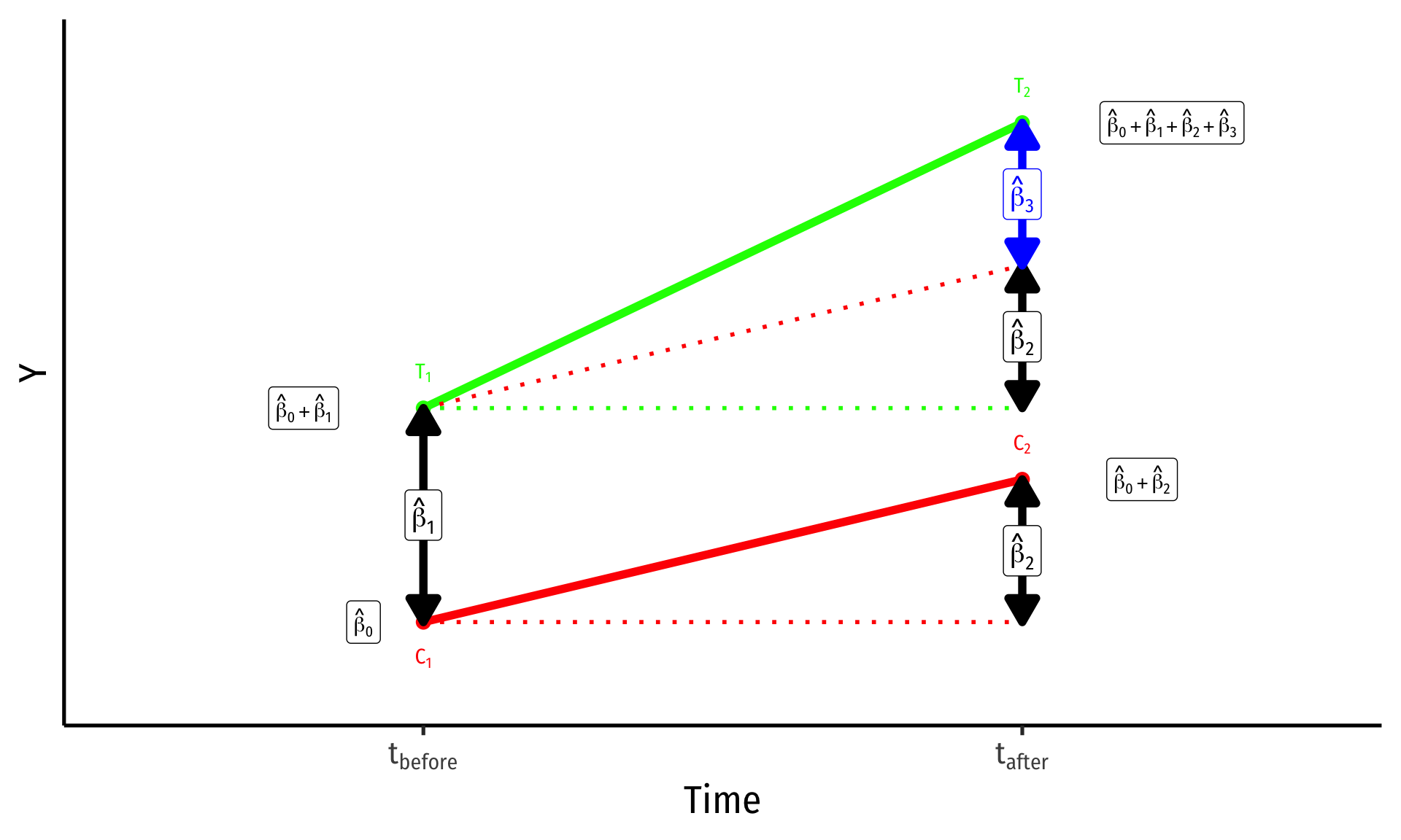
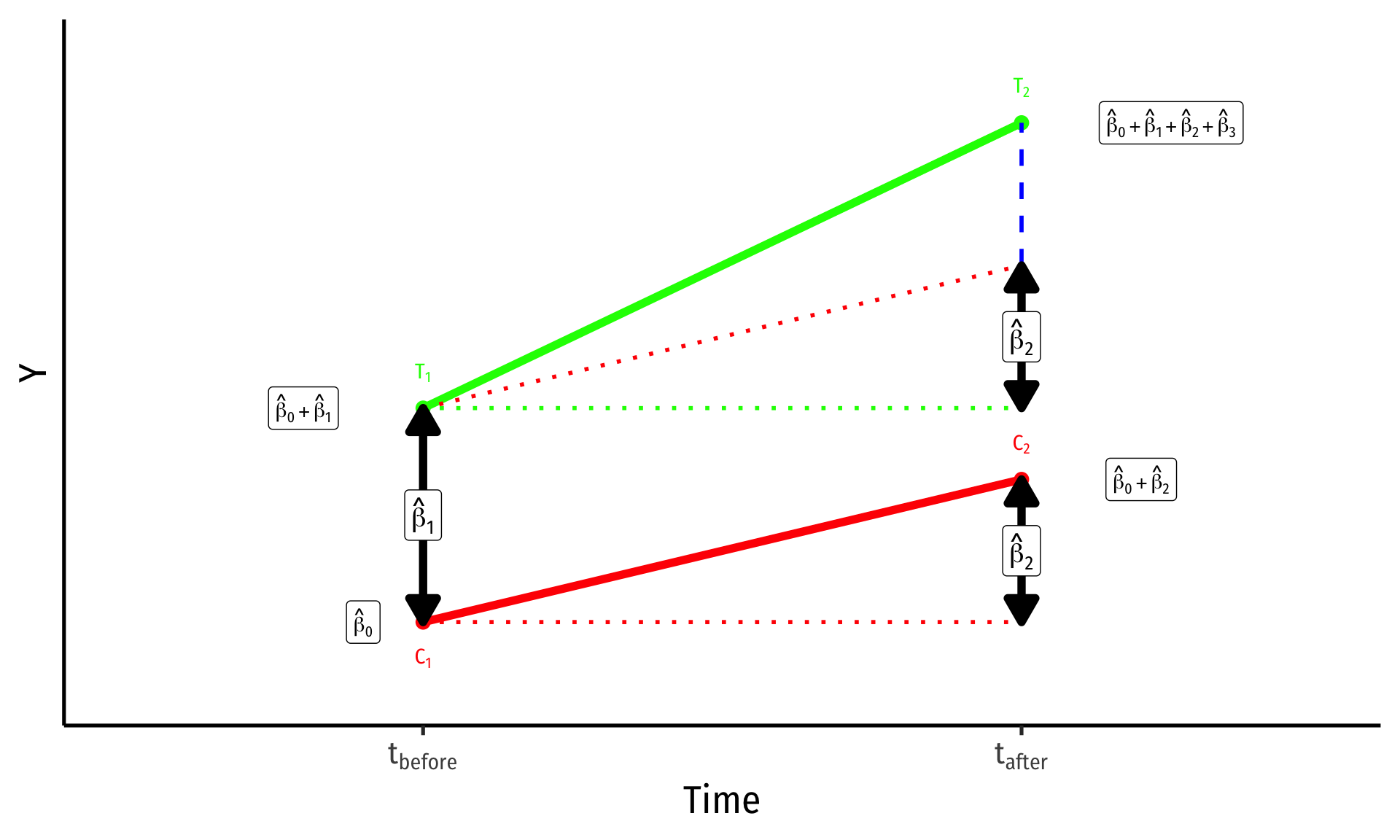
\(\bar{Y_i}\) for Control group before: \(\hat{\beta_0}\)
\(\bar{Y_i}\) for Control group after: \(\hat{\beta_0}+\hat{\beta_2}\)
\(\bar{Y_i}\) for Treatment group before: \(\hat{\beta_0}+\hat{\beta_1}\)
\(\bar{Y_i}\) for Treatment group after: \(\hat{\beta_0}+\hat{\beta_1}+\hat{\beta_2}+\hat{\beta_3}\)
Group Difference (before): \(\hat{\beta_1}\)
Time Difference: \(\hat{\beta_2}\)
Difference-in-differences: \(\hat{\beta_3}\) (treatment effect)
Key Assumption: Counterfactual
\[\hat{Y}_{it}=\beta_0+\beta_1 \, \text{Treated}_i +\beta_2 \, \text{After}_{t}+\beta_3 \,(\text{Treated}_i \times \text{After}_{t})+u_{it}\]
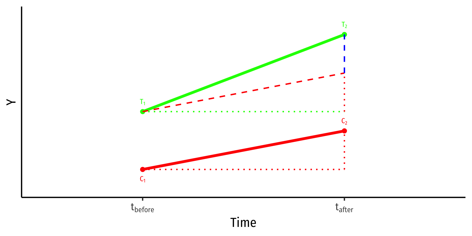
Key assumption for DND: time trends (for treatment and control) are parallel
Treatment and control groups assumed to be identical over time on average, except for treatment
Counterfactual: if the treatment group had not recieved treatment, it would have changed identically over time as the control group \((\hat{\beta_2})\)
Key Assumption: Counterfactual
\[\hat{Y}_{it}=\beta_0+\beta_1 \, \text{Treated}_i +\beta_2 \, \text{After}_{t}+\beta_3 \,(\text{Treated}_i \times \text{After}_{t})+u_{it}\]
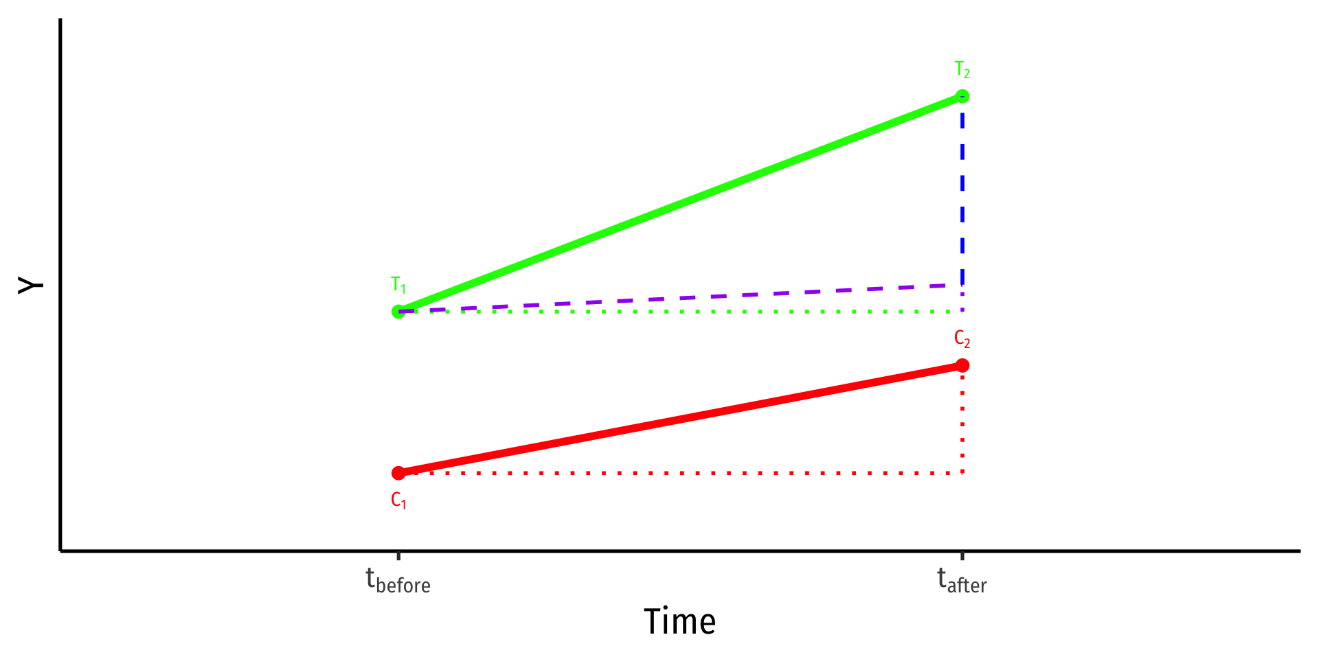
- If the time-trends would have been different, a biased measure of the treatment effect \((\hat{\beta_3})\)!
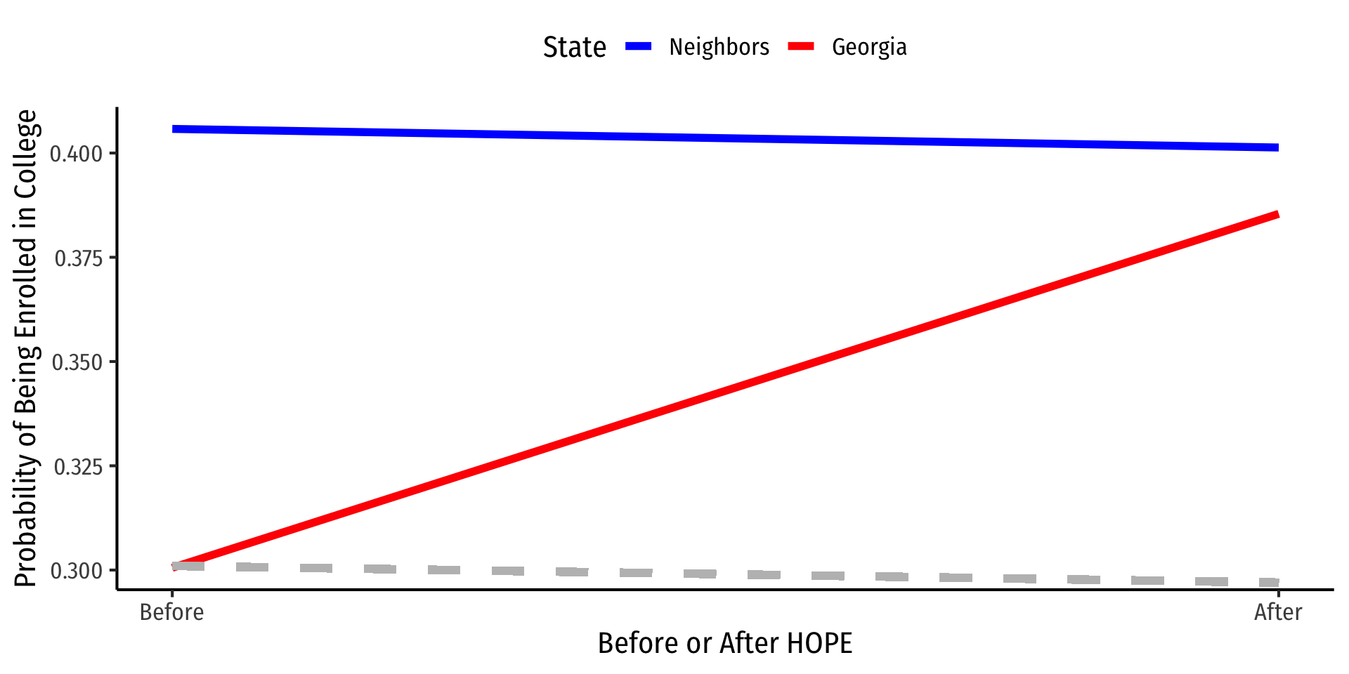
Example: Data
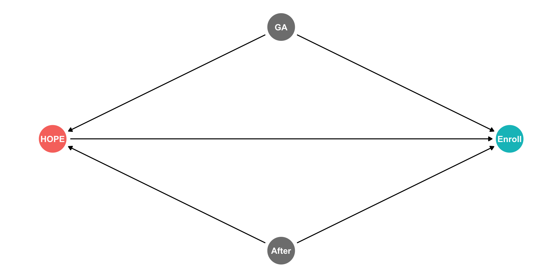
Dynarski, Susan, 1999, “Hope for Whom? Financial Aid for the Middle Class and its Impact on College Attendance,” National Tax Journal 53(3): 629-661
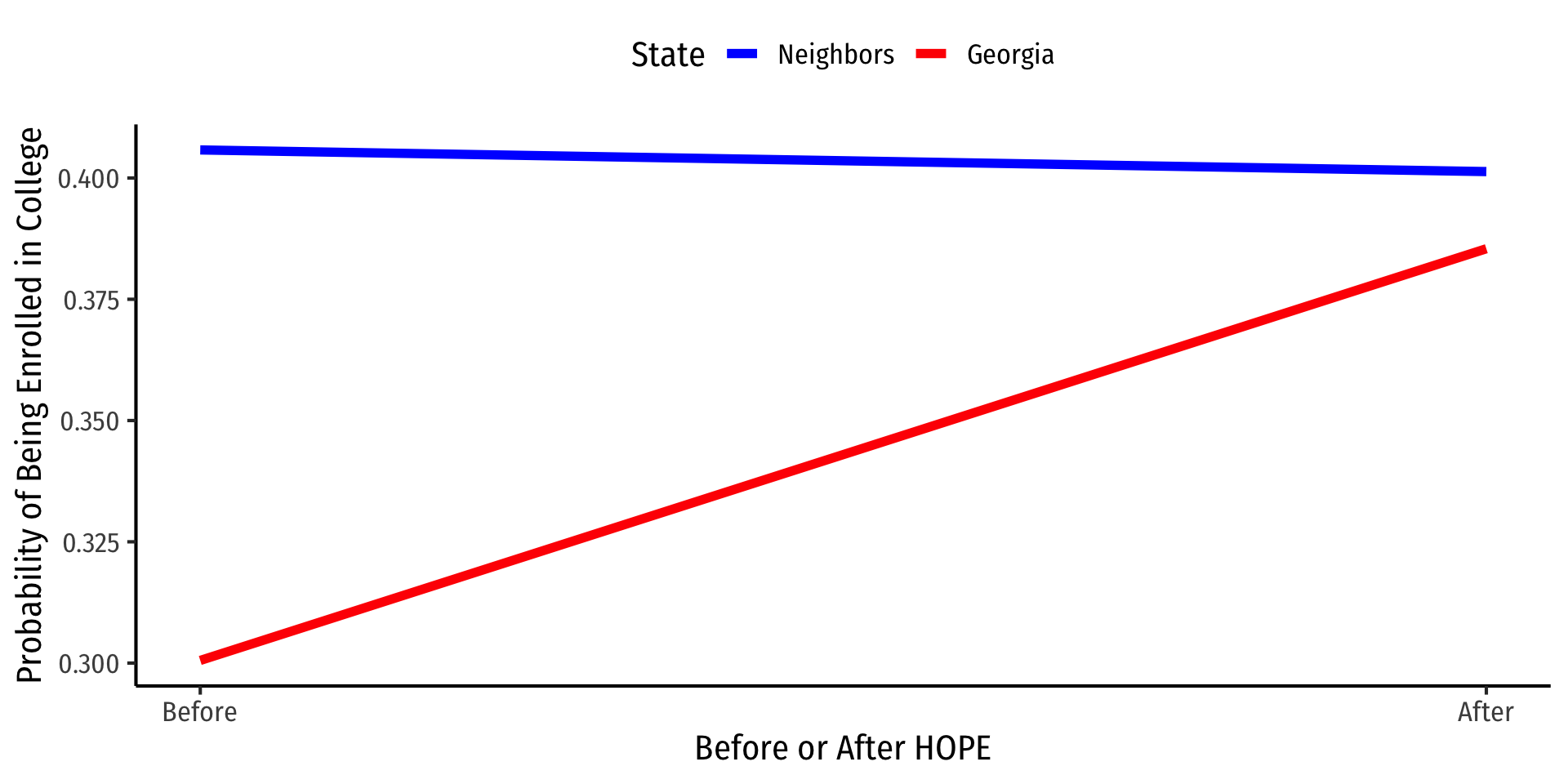
Diff-in-Diff Summary & Data
Dynarski, Susan, 1999, “Hope for Whom? Financial Aid for the Middle Class and its Impact on College Attendance,” National Tax Journal 53(3): 629-661
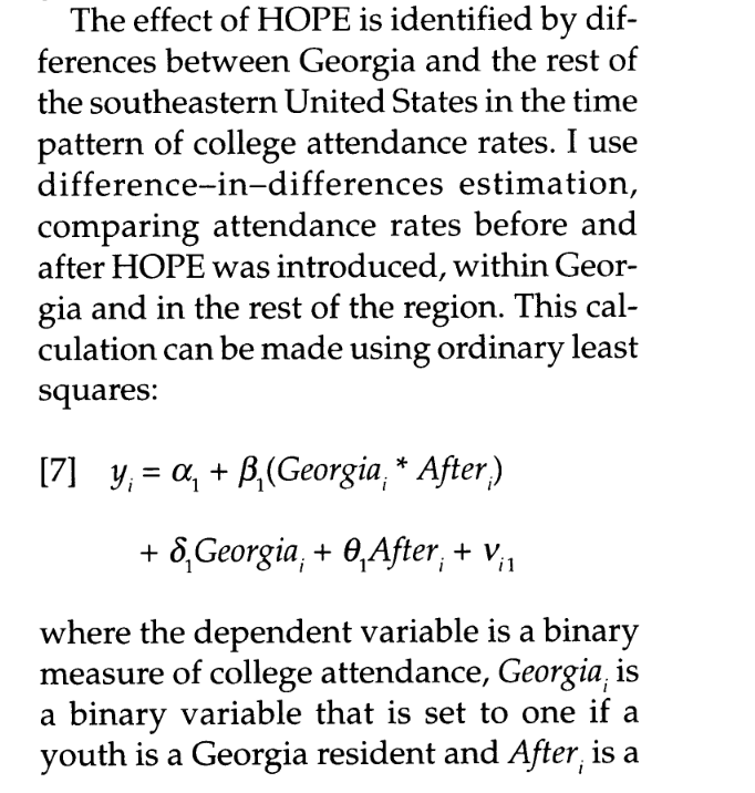
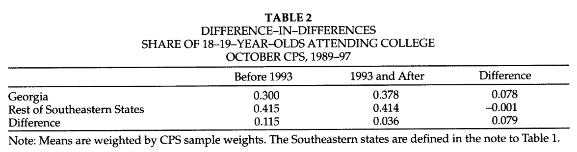
Example: Diff-in-Diff Graph
Example: Diff-in-Diff Graph
The Findings
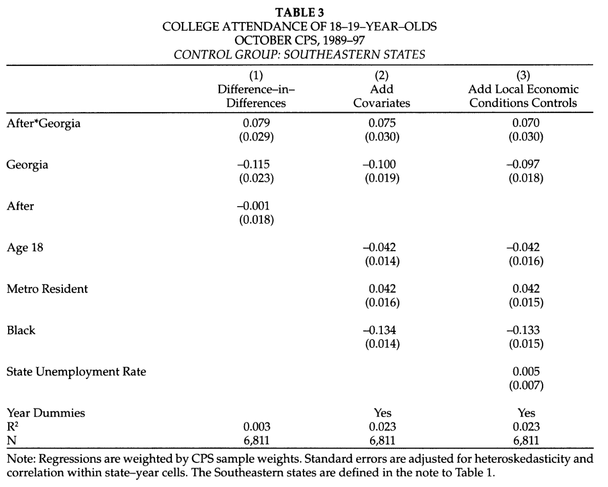
Dynarski, Susan, 1999, “Hope for Whom? Financial Aid for the Middle Class and its Impact on College Attendance,” National Tax Journal 53(3): 629-661
Intuition behind DND
Diff-in-diff models are the quintessential example of exploiting natural experiments
A major change at a point in time (change in law, a natural disaster, political crisis) separates groups where one is affected and another is not—identifies the effect of the change (treatment)
One of the cleanest and clearest causal identification strategies
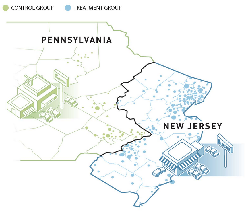
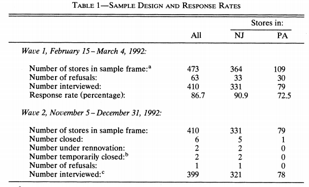
Card & Kreuger (1994): Background I
Card & Kreuger (1994) compare employment in fast food restaurants on New Jersey and Pennsylvania sides of border between February and November 1992.
Pennsylvania & New Jersey both had a minimum wage of $4.25 before February 1992
In February 1992, New Jersey raised minimum wage from $4.25 to $5.05
Card & Kreuger (1994): Background II
- If we look only at New Jersey before & after change:
- Omitted variable bias: macroeconomic variables (there’s a recession!), weather, etc.
- Including PA as a control will control for these time-varying effects if they are national trends
- Omitted variable bias: macroeconomic variables (there’s a recession!), weather, etc.
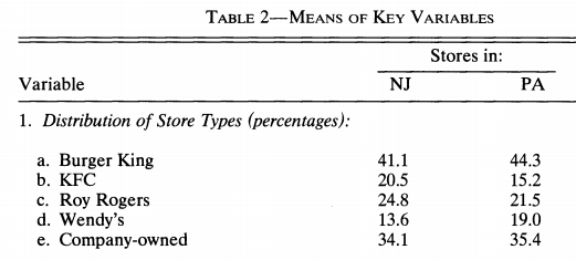
- Surveyed 400 fast food restaurants on each side of the border, before & after min wage increase
- Key assumption: Pennsylvania and New Jersey follow parallel trends,
- Counterfactual: if not for the minimum wage increase, NJ employment would have changed similar to PA employment
- Key assumption: Pennsylvania and New Jersey follow parallel trends,
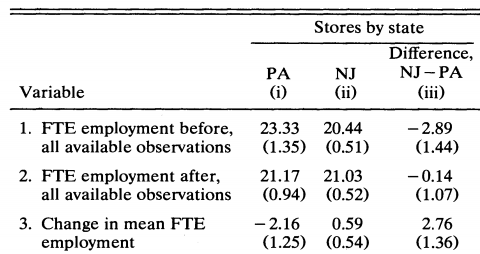
Card & Kreuger (1994): Comparisons
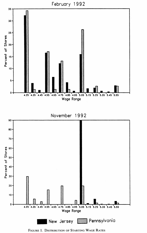
Card & Kreuger (1994): Summary I
Card & Kreuger (1994): Summary II
Card & Kreuger (1994): Results