Clever Research Designs Identify Causality
Again, this toolkit of research designs to identify causal effects is the economist’s comparative advantage that firms and governments want!
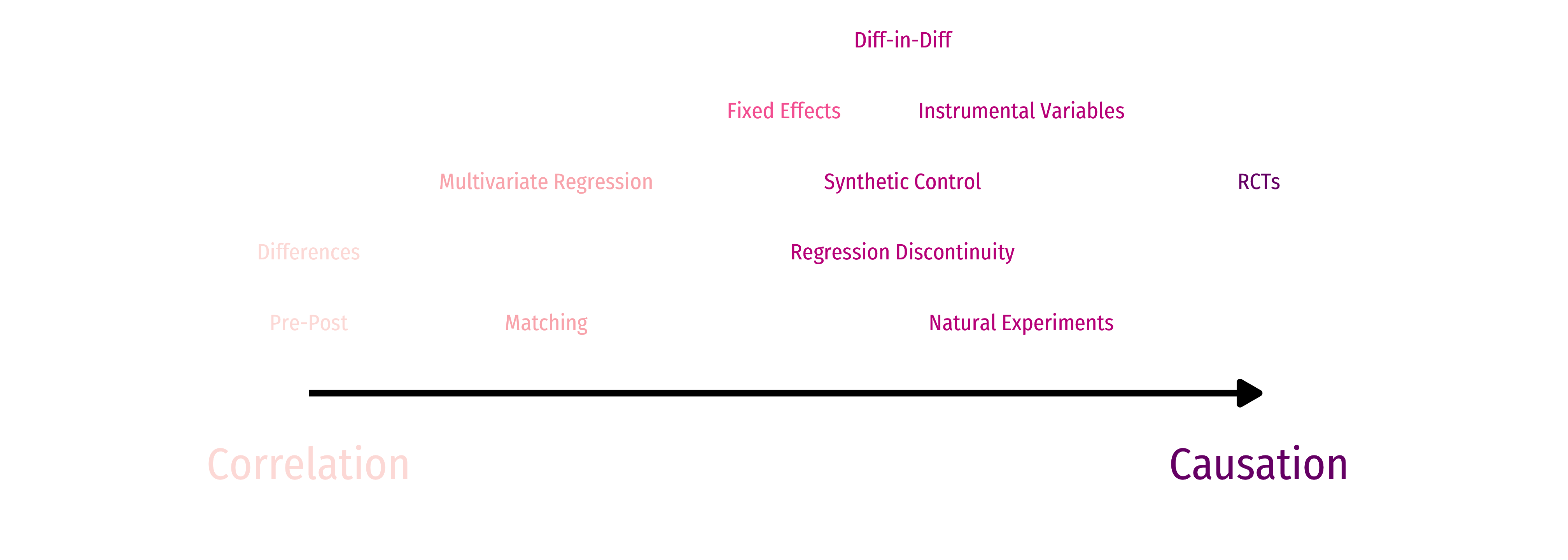
Identification Strategies
Endogeneity remains the hardest (and most common) econometric challenge
Diff-n-diff/fixed effects are one strategy to minimize endogeneity
- Requires panel data
- Can’t use time-varying omitted variables that are correlated with regressors
Another strategy to is to find some source of exogenous variation that removes the endogeneity of a variable, using that source as a instrumental variable

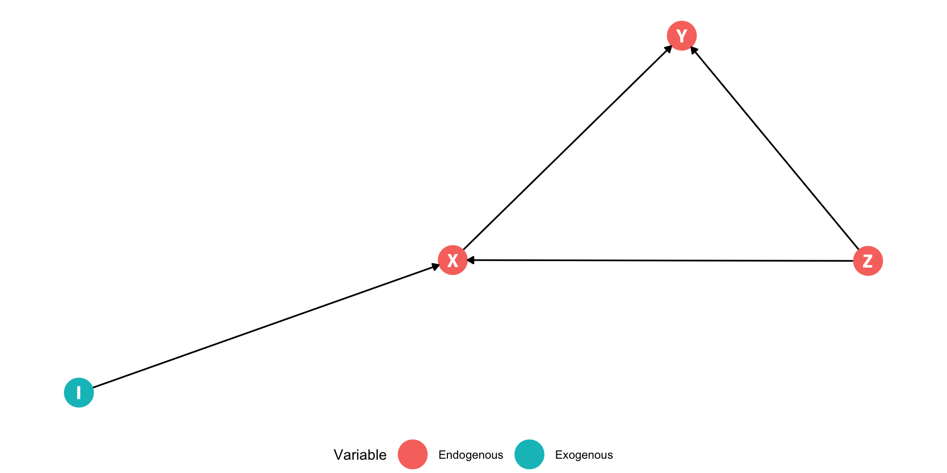
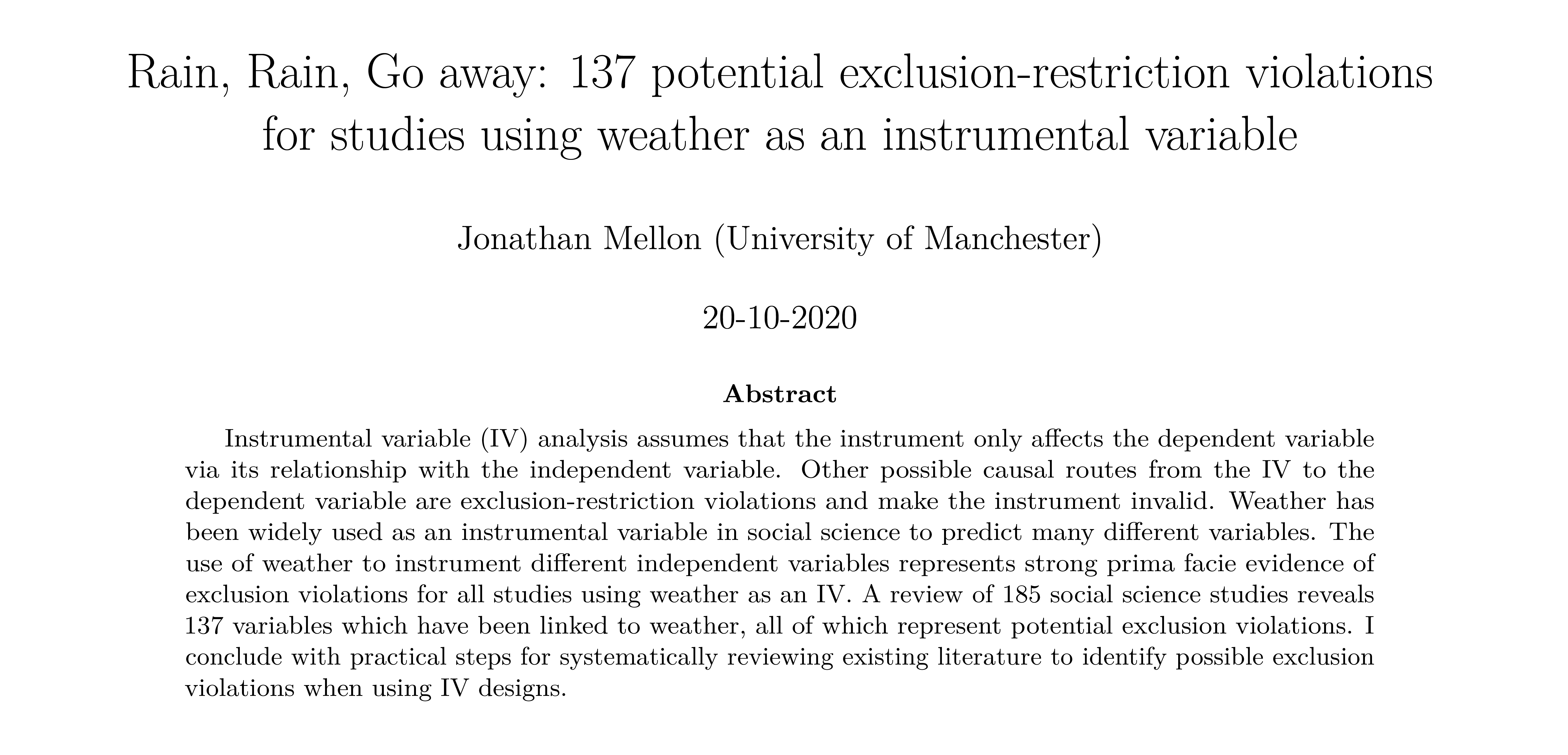
Understanding Instruments

Variable I has no backdoors between it and \(Y\)
The only way to reach \(Y\) from \(I\) is through \(X\):
- \(I \rightarrow X \rightarrow Y\)
Variable I is a good instrument for \(X\) if it satisfies two conditions:
- Inclusion condition: \(I\) statistically-significantly explains \(X\)
- Exclusion condition: \(I\) is uncorrelated with \(u\), so it does not directly affect \(Y\)
- \(I\) only affects \(Y\) through its effect on \(X\)
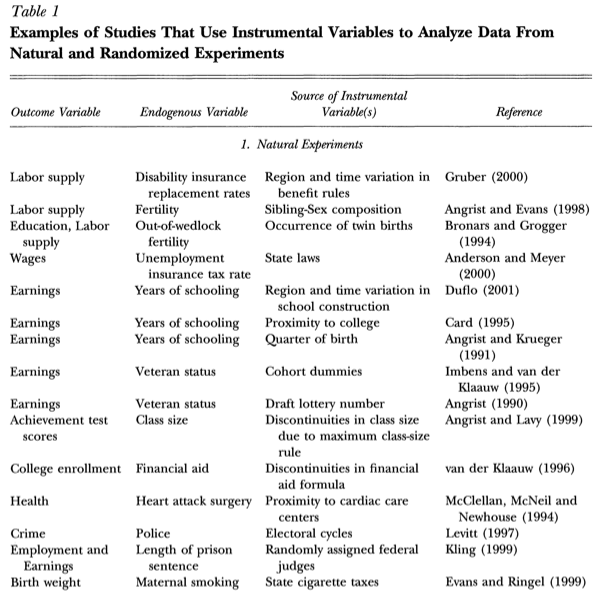
Example I: Veterans’ Earnings
Example
How does veteran status affect lifetime earnings?
\[\text{Earnings}_{i}=\beta_0+\beta_1 \, \text{Veteran}_{i}+\text{u}_{i}\]
- \(\text{Veteran}_i\) is endogenous, correlated with other things in \(u_i\)
- Choice to enlist in military for non-random reasons

Exogeneity: The “Huh?” Factor
“A necessary but not a sufficient condition for having an instrument that can satisfy the exclusion restriction is if people are confused when you tell them about the instrument’s relationship to the outcome,” (p.123).
Cunningham, Scott, 2021, Causal Inference: The Mixtape
Good Instruments are Hard to Find (And Weird) II
Angrist, Joshua D and Alan B Kreuger, 2001, “Instrumental Variables and the Search for Identification: From Supply and Demand to Natural Experiments,” Journal of Economic Perspectives 15(4): 69-85
Exogeneity: The “Huh?” Factor
“Remember what I said about how instruments having a certain ridiculousness to them? That is, you know you have a good instrument if the instrument itself doesn’t seem relevant for explaining the outcome of interest because that’s what the exclusion restriction implies. Why would quarter of birth affect earnings? It doesn’t make any obvious, logical sense why it should. But, if I told you that people born later in the year got more schooling than those with less because of compulsory schooling, then the relationship between the instrument and the outcome snaps into place. The only reason we can think of as to why the instrument would affect earnings is if the instrument were operating through schooling. Instruments only explain the outcome, in other words, when you understand their effect on the endogenous variable,” (p.123).
Cunningham, Scott, 2021, Causal Inference: The Mixtape
Good Instruments are Hard to Find (And Weird) III
“Testing” the Exclusion Restriction
- Can you argue that the instrument does not affect outcome \(Y\) except only through \(X\)?
Examples
- Instrument \(\rightarrow\) ? \(\rightarrow\) outcome
- Quarter of birth \(\rightarrow\) ? \(\rightarrow\) wages
- Rainfall \(\rightarrow\) ? \(\rightarrow\) civil war
- Scrabble score of name \(\rightarrow\) ? \(\rightarrow\) wages
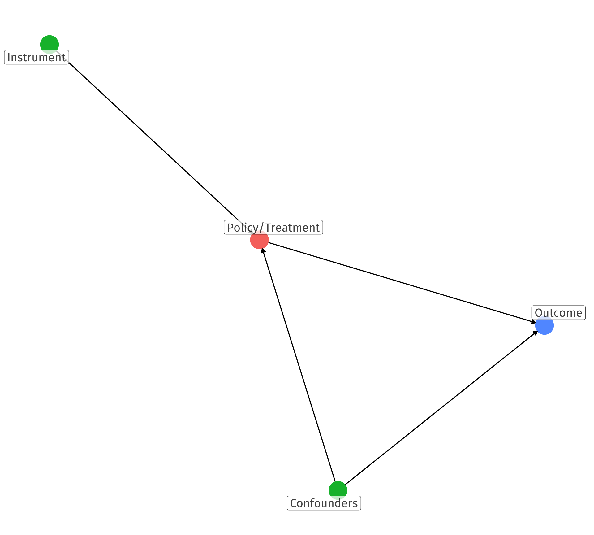
Example I: DAG Form

- Causal pathways from \(X\) to \(Y\):
- \(\color{red}{Vet} \rightarrow \color{green}{Earn}\)
- \(\color{red}{Vet} \leftarrow \color{blue}{U} \rightarrow \color{green}{Earn}\)
- We want the causal effect of
\[\color{red}{Vet} \rightarrow \color{green}{Earn}\]
- With our instrument
\[\color{blue}{Draft} \rightarrow \color{red}{Vet} \rightarrow \color{green}{Earn}\]
Example I: DAG Form
- With our instrument
\[\color{blue}{Draft} \rightarrow \color{red}{Vet} \rightarrow \color{green}{Earn}\]
- Based on our assumptions on independence and exogeneity:
(Effect of draft on earnings) \(=\)
(Effect of draft on veteran) \(\times\) (Effect of veteran on earnings)
Example I: DAG Form

- With our instrument
\[\color{blue}{Draft} \rightarrow \color{red}{Vet} \rightarrow \color{green}{Earn}\]
- Based on our assumptions on independence and exogeneity:
(Effect of draft on earnings) \(=\)
(Effect of draft on veteran) \(\times\) (Effect of veteran on earnings)
- To find effect of veteran on earnings, rearrange!
(Effect of veteran on earnings) \(=\)
(Effect of draft on earnings)
(Effect of draft on veteran)
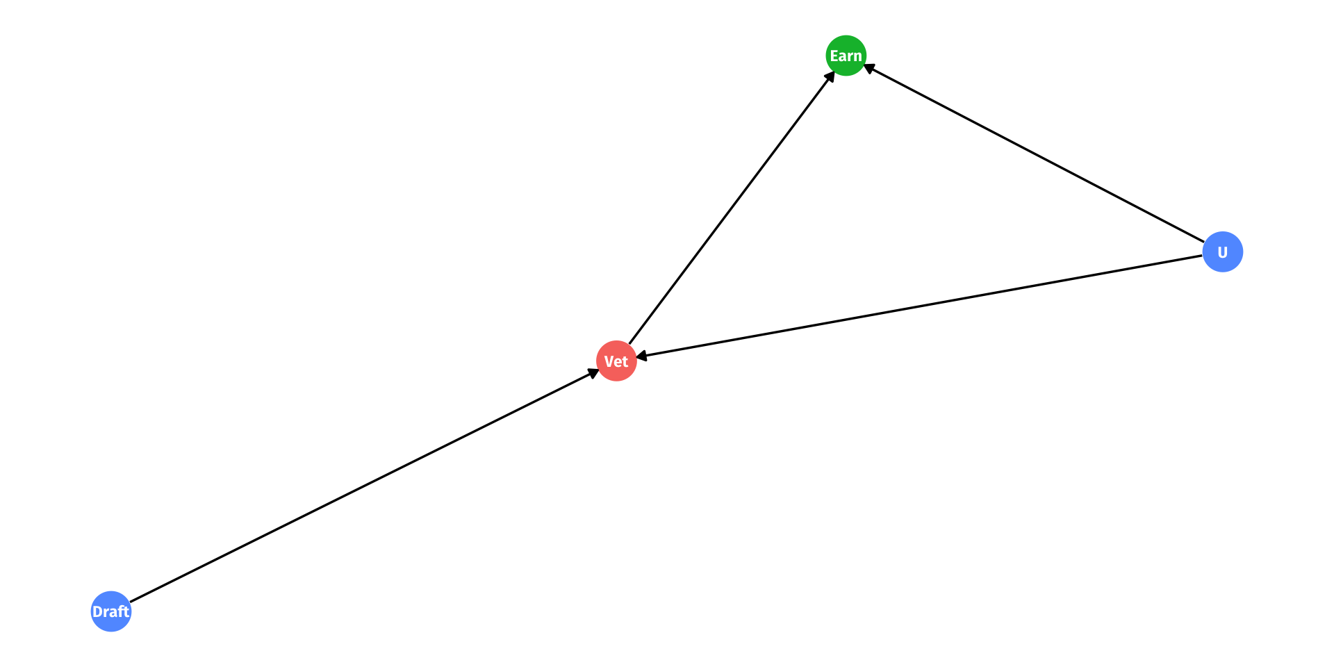
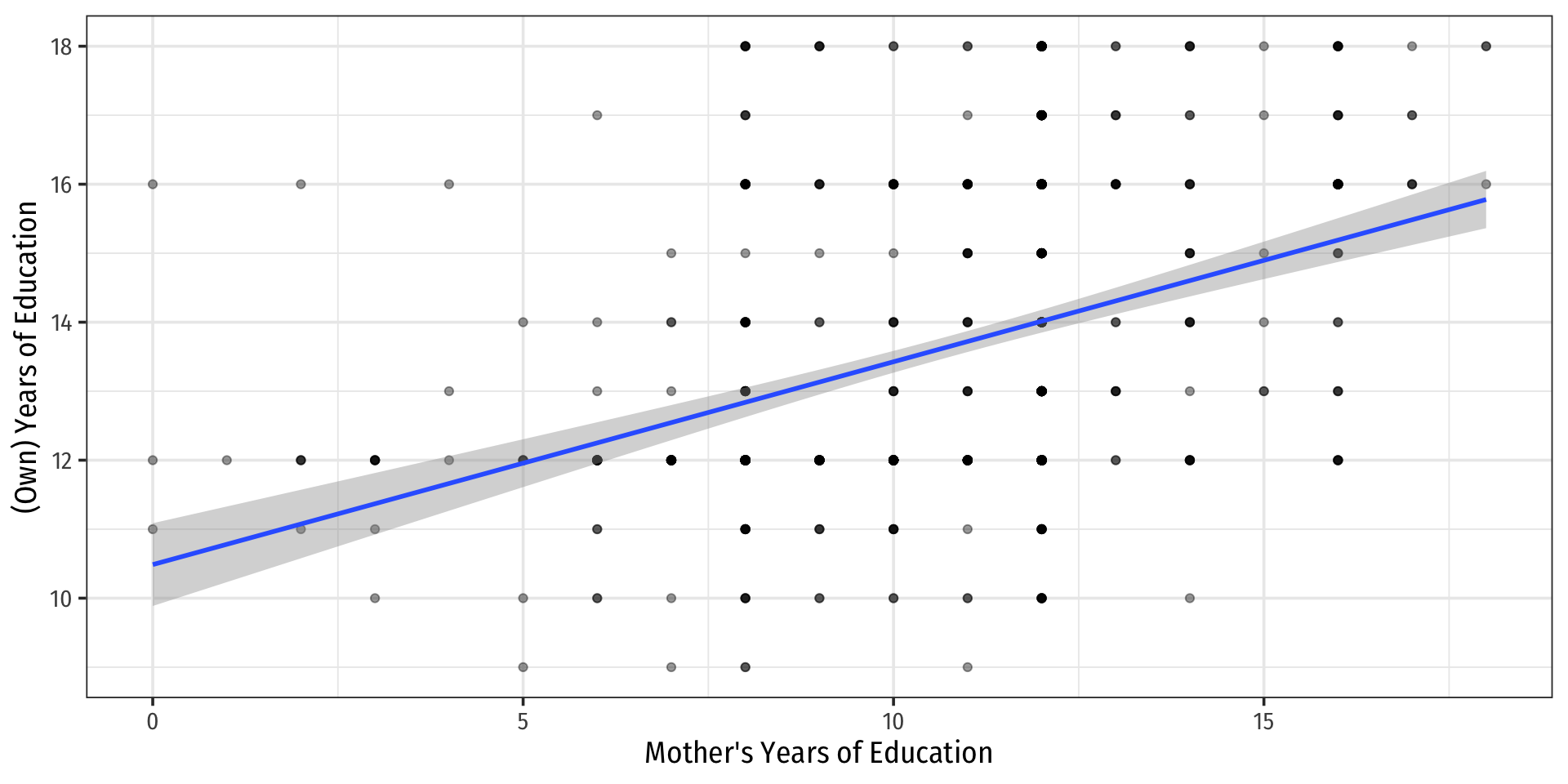
Example: Instrument
- Causal pathways from \(educ\) to \(wage\):
- \(\color{red}{educ} \rightarrow \color{green}{wage}\)
- \(\color{red}{educ} \leftarrow \color{blue}{U} \rightarrow \color{green}{wage}\)
- We want the causal effect of
\[\color{red}{educ} \rightarrow \color{green}{wage}\]
- With our instrument
\[\color{blue}{mom} \rightarrow \color{red}{educ} \rightarrow \color{green}{wage}\]
First-Stage Visualized
Another Example: Levitt (2002) IV
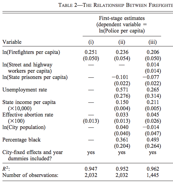
Instrument is statistically significant (\(t \approx 5\)), inclusion condition met
A 1% increase in firefighters is associated with a 0.206-0.251% increase in police
Another Example: Levitt (2002) V
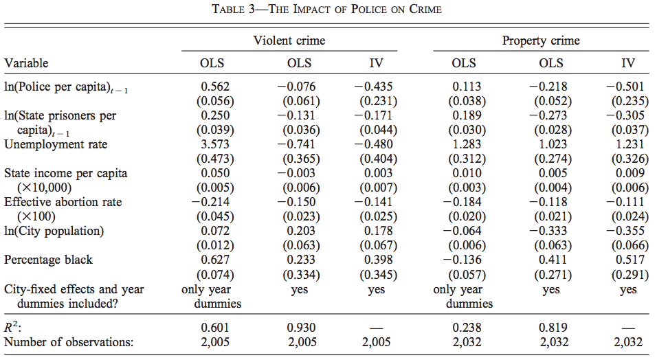
A 1% increase in police (last year) leads to a 0.435% decrease in violent crimes, 0.501% decrease in property crimes
Another Example: AJR (2001) I
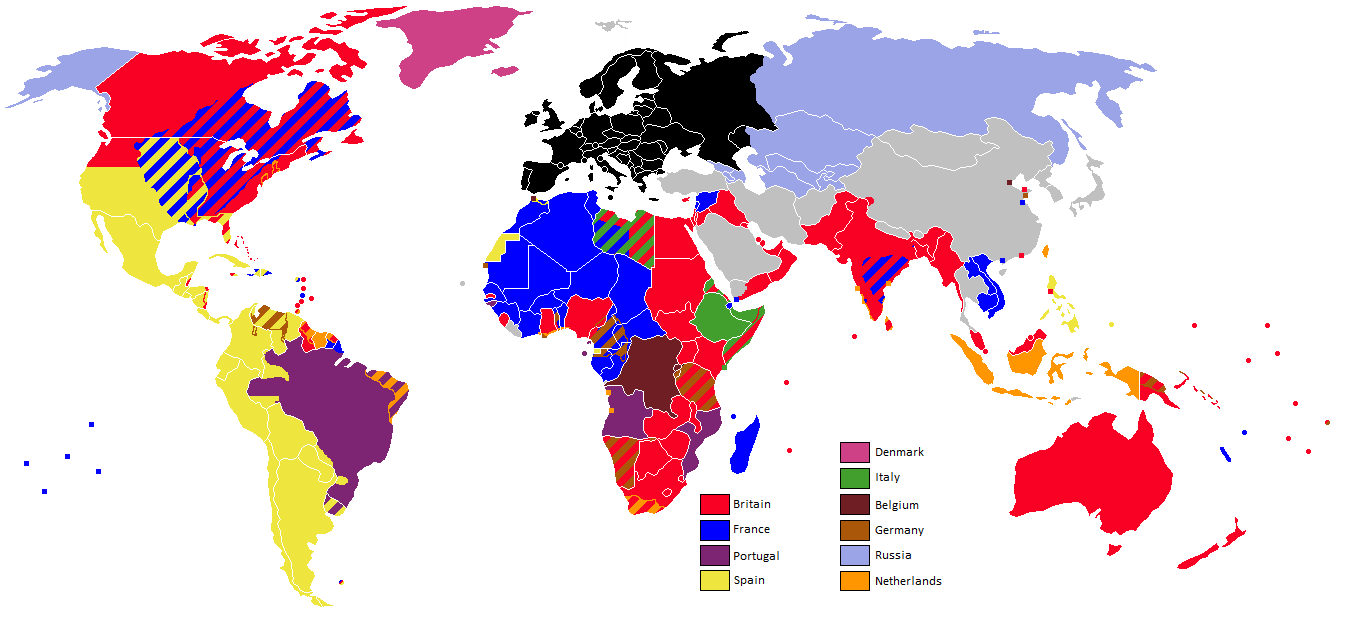
Another Example: AJR (2001) III
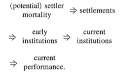
- Instrument: Settler Mortality in 1500
- Inclusion Restriction: Settler mortality in 1500 determines risk of expropriation today
- {Exclusion Restriction: Settler mortality in 1500 does not affect Present GDP
- Settler mortality in 1500 only affects Present GDP through institutions determined by historical path set by settler mortality rates
Acemoglu, Daron, Simon Johnson, and James A Robinson, (2001), “The Colonial Origins of Comparative Development: An Empirical Investigation,” American Economic Review 91(5): 1369-1401
Another Example: AJR (2001) V
Relationship Between \(Y\) and \(IV\)
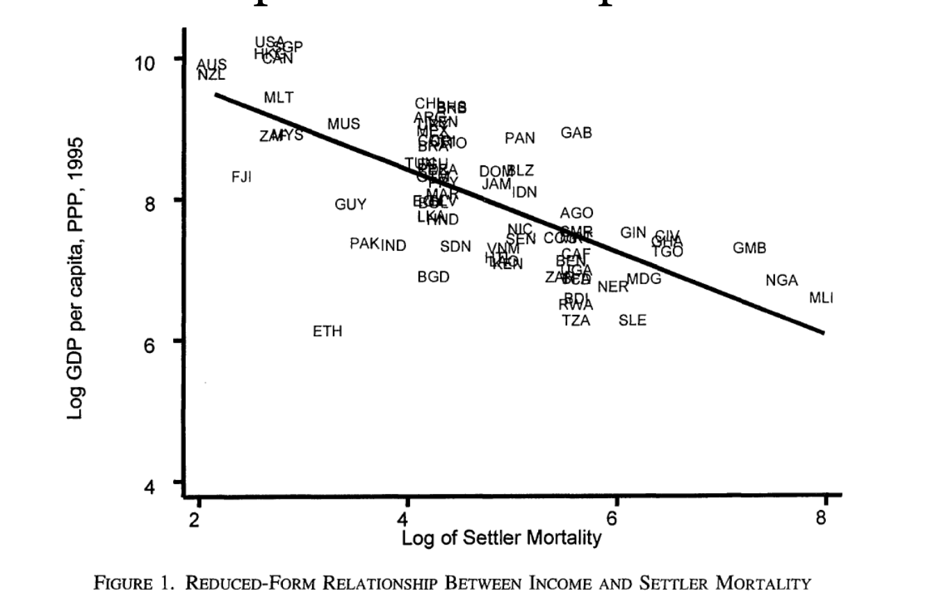
Another Example: AJR (2001) VI
Relationship Between \(X\) and \(Y\)
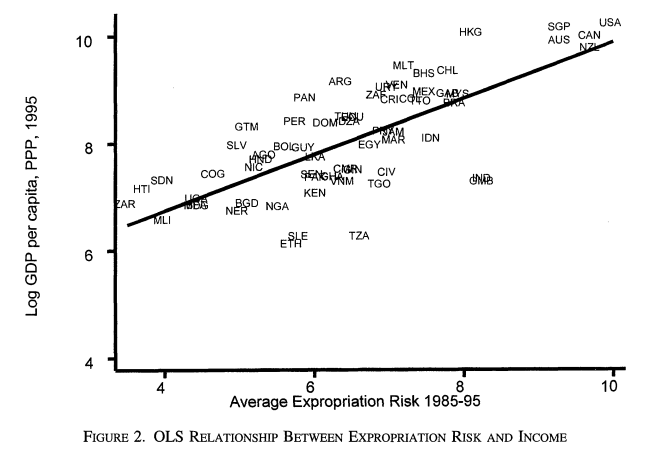
Another Example: AJR (2001) VII
Relationship Between \(X\) and \(IV\)
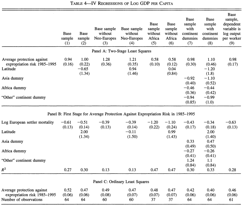
Another Example: AJR (2001) VIII
2SLS Results
Supply and Demand
A famous example, foundational to our discipline, Supply and Demand
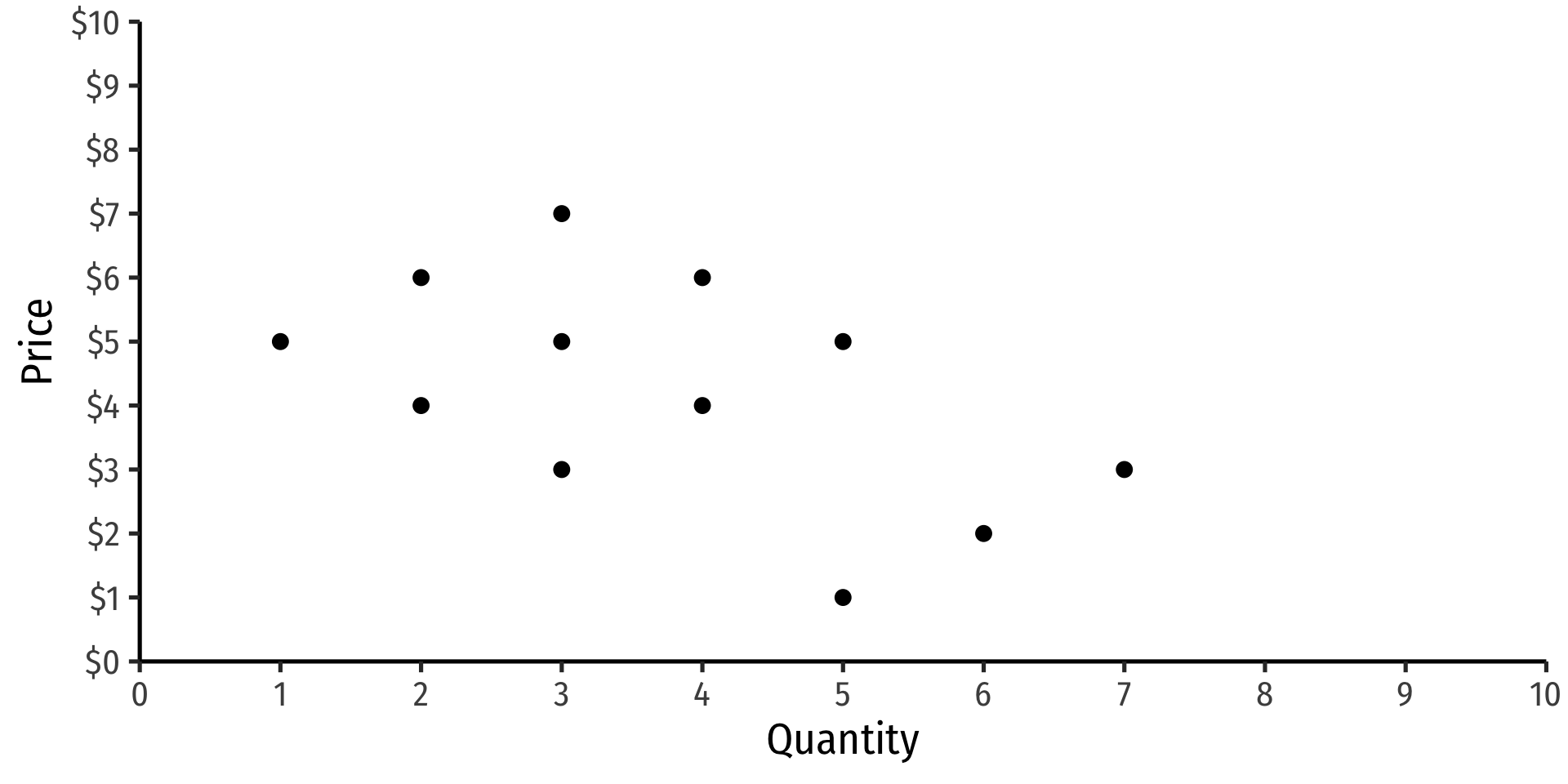
Suppose you have data on price and quantity, and want to estimate a Demand curve with regression
Supply and Demand
A famous example, foundational to our discipline, Supply and Demand
Suppose you have data on price and quantity, and want to estimate a Demand curve with regression
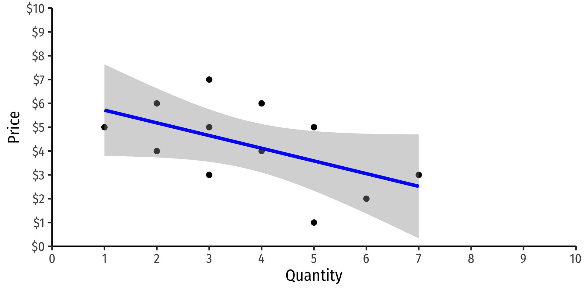
Why can’t we estimate the demand curve with a simple regression here?
\[\ln(\text{Quantity}_{it}) = \beta_0 + \beta_1 \ln(\text{Price}_{it}) + u_{it}\]
- With natural logs, \(\beta_1\) is the price elasticity of Demand
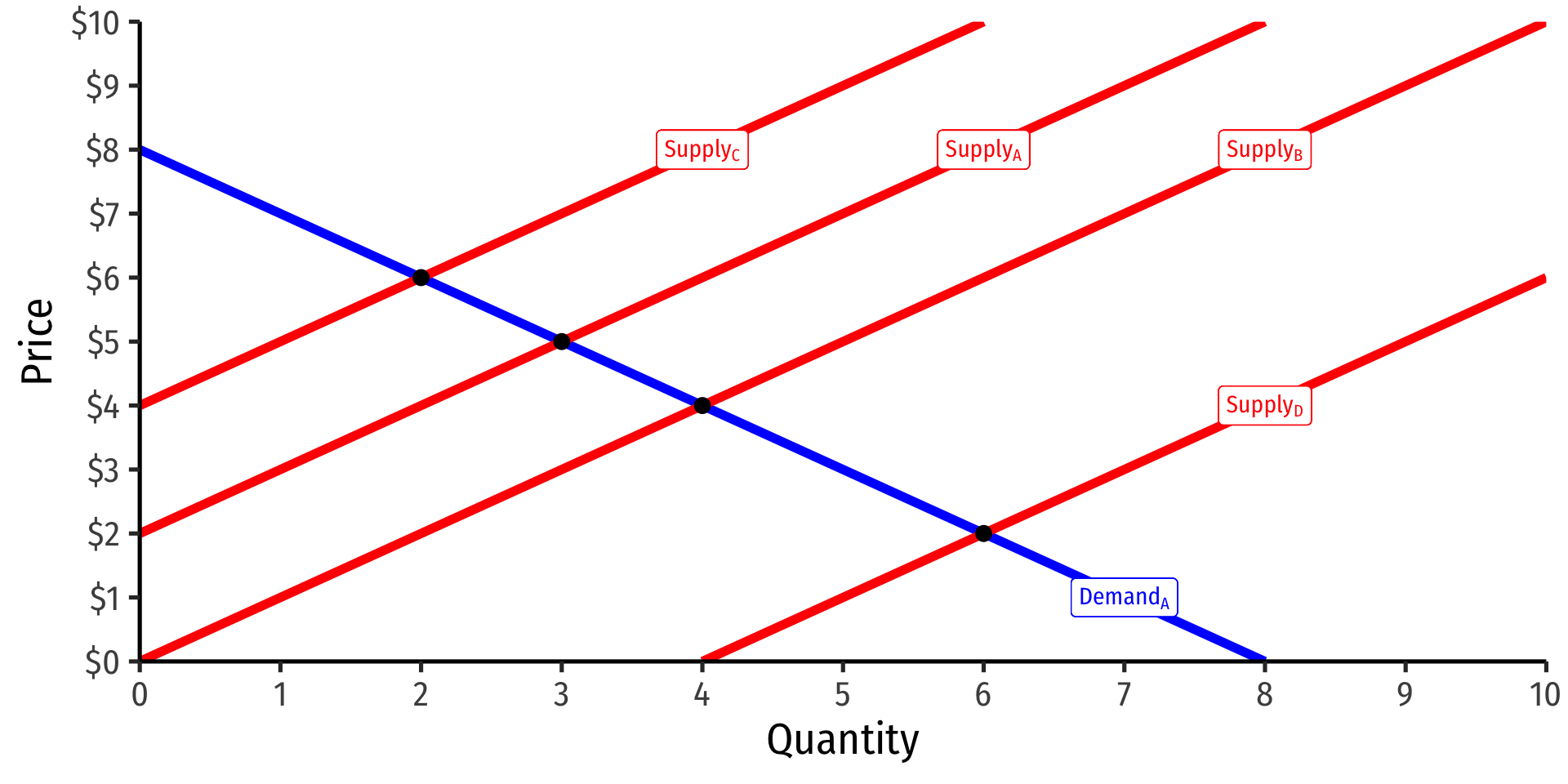
Supply and Demand: Simultaneous Causality
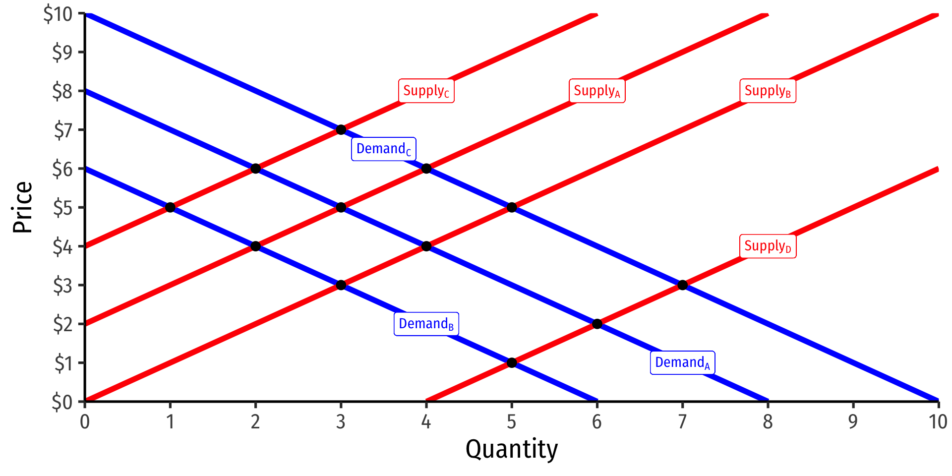
The data are actually all equilibrium \((Q^*,P^*)\) points!
Result of many demand and supply curve shifts & intersections!
Supply and Demand: Simultaneous Causality

\[\color{blue}{Q_D = \alpha_0 + \alpha_1 P + \alpha_2 M + u_D}\]
Why can’t we just estimate price elasticity of demand \((\alpha_1)\) with the demand equation?
\(P\) is partially a function of quantity supplied!
Supply and Demand: Simultaneous Causality
Instrumental variables can identify the demand relationship
Conceptually, use some supply shifter (like cost changes, \(\color{red}{C})\) correlated with price \(\color{blue}{P}\), but not correlated with \(\color{blue}{u_D}\)
Essentially: traces out unique demand relationship by allowing supply to vary & shift
Then, can estimate demand elasticity \(\beta_1\)
Demand Example

Demand Example 😨
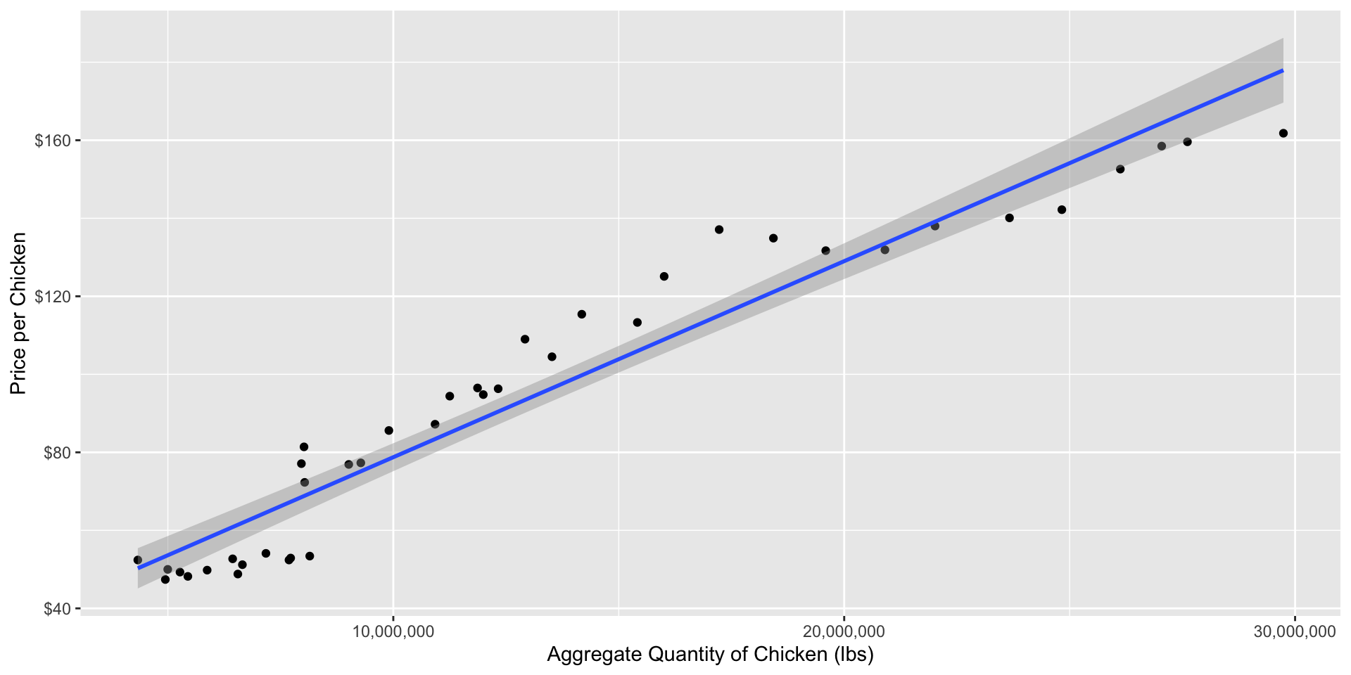
Consider the Causality
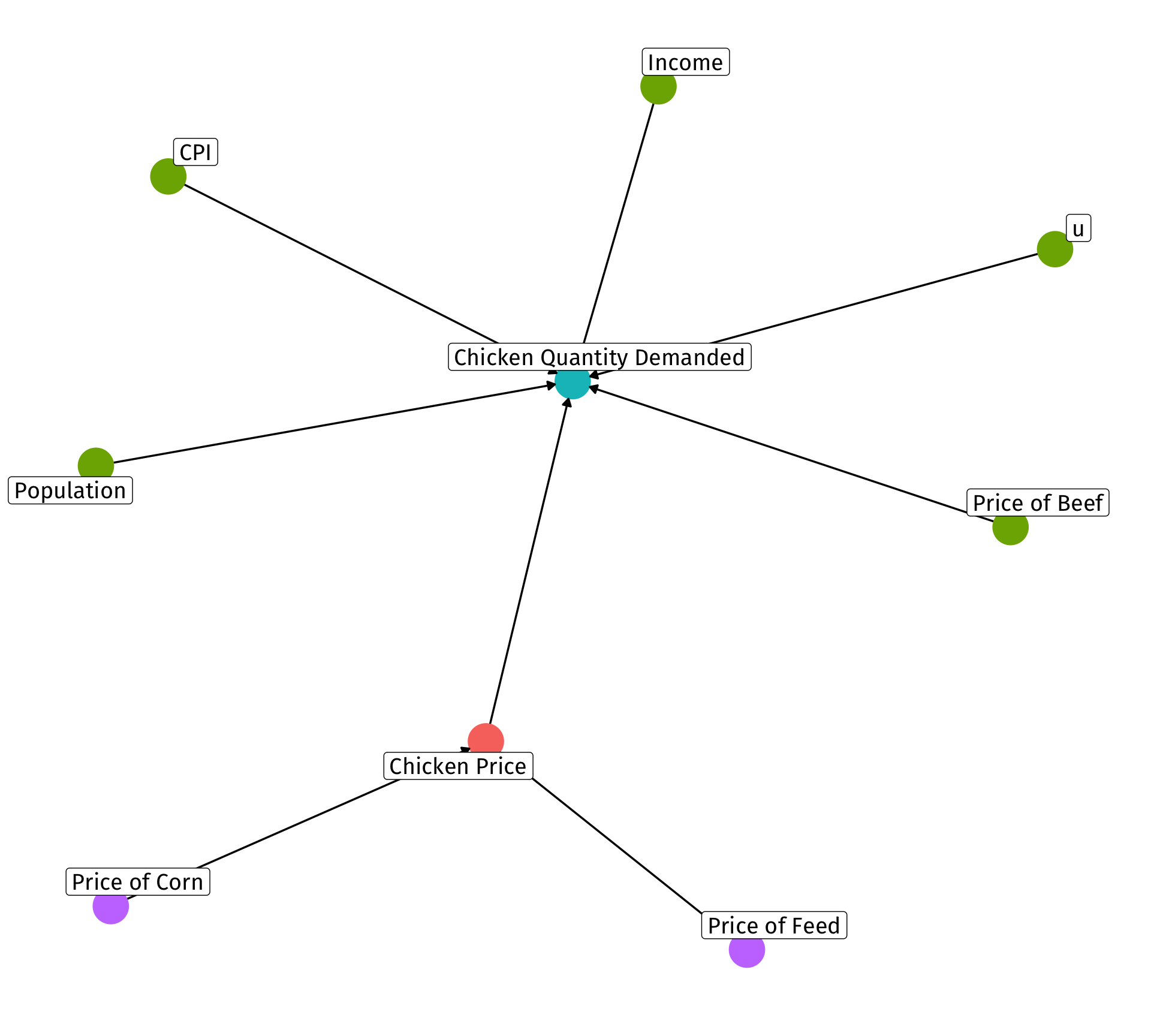
- Factors that influence quantity demanded:
- price (endogenous! — partly determined by supply!)
- price of substitutes (beef)
- income
- number of buyers (population)
- price level (CPI)
- other unobservables (u)
- Factors that influence price (on the supply side)
- price of inputs/costs (feed and corn)
- use these as instruments for price!
Comparing
| OLS | OLS | 2SLS (by hand) | 2SLS (fixest) | |
|---|---|---|---|---|
| Constant | 10.624*** | −3.292** | −2.687 | −2.687 |
| (0.244) | (1.576) | (1.691) | (1.721) | |
| Log Price/lb of Chicken | 1.258*** | −0.281*** | −0.438*** | −0.438** |
| (0.054) | (0.090) | (0.159) | (0.162) | |
| Log Income | 0.116 | 0.209 | 0.209 | |
| (0.217) | (0.235) | (0.240) | ||
| Log Price/lb of Beef | −0.049 | 0.004 | 0.004 | |
| (0.063) | (0.078) | (0.080) | ||
| Log Population | 3.593*** | 3.388*** | 3.388*** | |
| (0.595) | (0.633) | (0.644) | ||
| CPI | 0.005*** | 0.006*** | 0.006*** | |
| (0.001) | (0.001) | (0.001) | ||
| n | 40 | 40 | 40 | 40 |
| Adj. R2 | 0.93 | 1.00 | 1.00 | 1.00 |
| SER | 0.14 | 0.03 | 0.03 | 0.03 |
| * p < 0.1, ** p < 0.05, *** p < 0.01 |
