Midterm Concepts

OLS Regression

Bivariate data and associations between variables (e.g. $X$ and $Y$)

• Apparent relationships are best viewed by looking at a scatterplot

• Check for associations to be positive/negative, weak/strong, linear/nonlinear, etc

  • $Y$: dependent variable

  • $X$: independent variable

• Correlation coefficient ($r$) can quantify the strength of an association

  $$r_{X,Y}=\frac{1}{n-1}\sum ^n(\frac{X_i-\overline{X}}{s_X})(\frac{Y_i-\overline{Y}}{s_Y})=\frac{{\displaystyle \sum ^n{Z}_X{Z}_Y}}{n-1}$$

  • $-1\le r\le 1$ and $r$ only measures linear associations

  • $|r|$ closer to 1 imply stronger correlation (near a perfect straight line)

  • Correlation does not imply causation! Might be confounding or lurking variables (e.g.$Z$) affecting $X$ and/or $Y$

Population regression model

$$Y_i={\beta }_0+{\beta }_1{X}_i+u_i$$

• ${\beta }_1$: $\frac{\mathrm{\Delta }Y}{\mathrm{\Delta }X}$: the slope between $X$ and $Y$, number of units of $Y$ from a 1 unit change in $X$

• ${\beta }_0$ is the $Y$-intercept: literally, value of $Y$ when $X=0$

• $u_i$ is the error, difference between actual value of $Y|X$ vs. predicted value of $\hat{Y}$

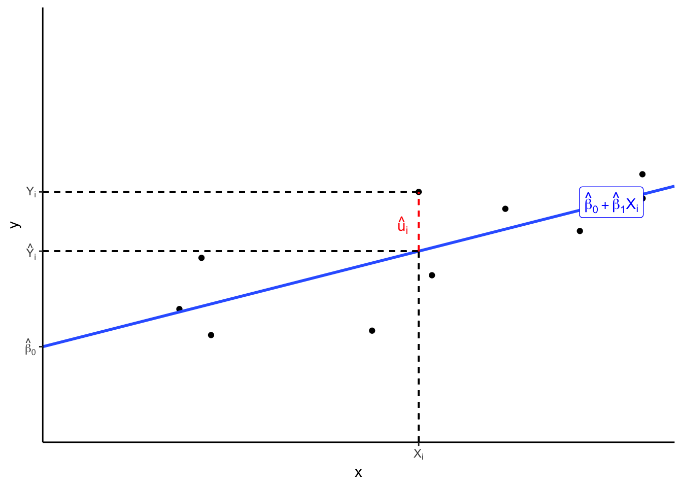
Ordinary Least Squares (OLS) regression model

$$Y_i={\hat{\beta }}_0+{\hat{\beta }}_1{X}_i+u_i$$

$$\widehat{Y_i}=\widehat{{\beta }_0}+\widehat{{\beta }_1}{X}_i$$

$${\hat{u}}_i=Y_i-{\hat{Y}}_i$$

• OLS estimators $\widehat{{\beta }_0}$ and $\widehat{{\beta }_1}$ estimate population regression line from sample data

• Minimize sum of squared errors (SSR) $min{\displaystyle \sum ^n{\hat{u}}_i^2}$

• OLS regression line

$$\widehat{{\beta }_1}=\frac{cov(X,Y)}{var(X)}=\frac{\sum (X_i-\overline{X})(Y_i-\overline{Y})}{\sum (X_i-\overline{X}{)}^2}=r_{X,Y}\frac{s_Y}{s_X}$$

$$\widehat{{\beta }_0}=\overline{Y}-\widehat{{\beta }_1}\overline{X}$$

Measures of Fit

• $R^2$: fraction of total variation on $Y$ explained by variation in $X$ according to model

$$\begin{array}{rl}{R}^2& =\frac{SSM}{SST}\\ R^2& =1-\frac{SSR}{SST}\\ R^2& =r_{X,Y}^2\end{array}$$

• Where

  • $SSM=\sum ({\hat{Y}}_i-{\overline{Y}}_i{)}^2$

  • $SST=\sum (Y_i-{\overline{Y}}_i{)}^2$

  • $SSR=\sum u_i^2$

• Standard error of the regression (or residuals), SER: average size of ${\hat{u}}_i$, i.e. average distance between points and the regression line

  $$SER({\sigma }_{{\hat{u}}_i})=\frac{SSR}{n-2}=\frac{\sum {\widehat{u_i}}^2}{n-2}$$

Sampling Distribution of ${\hat{\beta }}_1$

$\widehat{{\beta }_1}$ is a random variable, so it has its own sampling distribution with mean $\mathbb{E}[\widehat{{\beta }_1}]$ and standard error $se[\widehat{{\beta }_1}]$

• Mean of OLS estimator $\widehat{{\beta }_1}$ & Bias: Endogeneity & Exogeneity

  • $X$ is exogenous if it is not correlated with the error term

    $$\begin{array}{rl}cor(X,u)& =0\\ \mathbb{E}[u|X]& =0\end{array}$$

    • equivalently, knowing $X$ should tell us nothing about $u$ (zero conditional mean assumption)

    • if $X$ is exogenous, OLS estimate of ${\beta }_1$ is unbiased

      $$E[{\hat{\beta }}_1]={\beta }_1$$

  • $X$ is endogenous if it is correlated with the error term

    $$cor(X,u)\ne 0$$

    • If $X$ is endogenous, OLS estimate of ${\beta }_1$ is biased:

      $$\mathbb{E}[{\hat{\beta }}_1]={\beta }_1+\underset{bias}{\underbrace{cor(X,u)\frac{{\sigma }_u}{{\sigma }_X}}}$$

      • Can measure strength and direction (+ or -) of bias

      • Note if unbiased, $cor(X,u)=0$, so $E[\widehat{{\beta }_1}]={\beta }_1$

  • Assumptions about u

    1. The mean of the errors is 0

       $$\mathbb{E}[u_i]=0$$

    2. The variance of the errors is constant over all values of $X$ (homoskedasticity)

       $$var[u_i|X_i]={\sigma }_u^2$$

    3. Errors are not correlated across observations $i$ and $j$ (no autocorrelation)

       $$cor(u_i,u_j)=0$$

    4. There is no correlation between $X$ and $u$, i.e. the model is exogenous

       $$\begin{array}{rl}cor(X,u)& =0\\ \mathbb{E}[u|X]& =0\end{array}$$

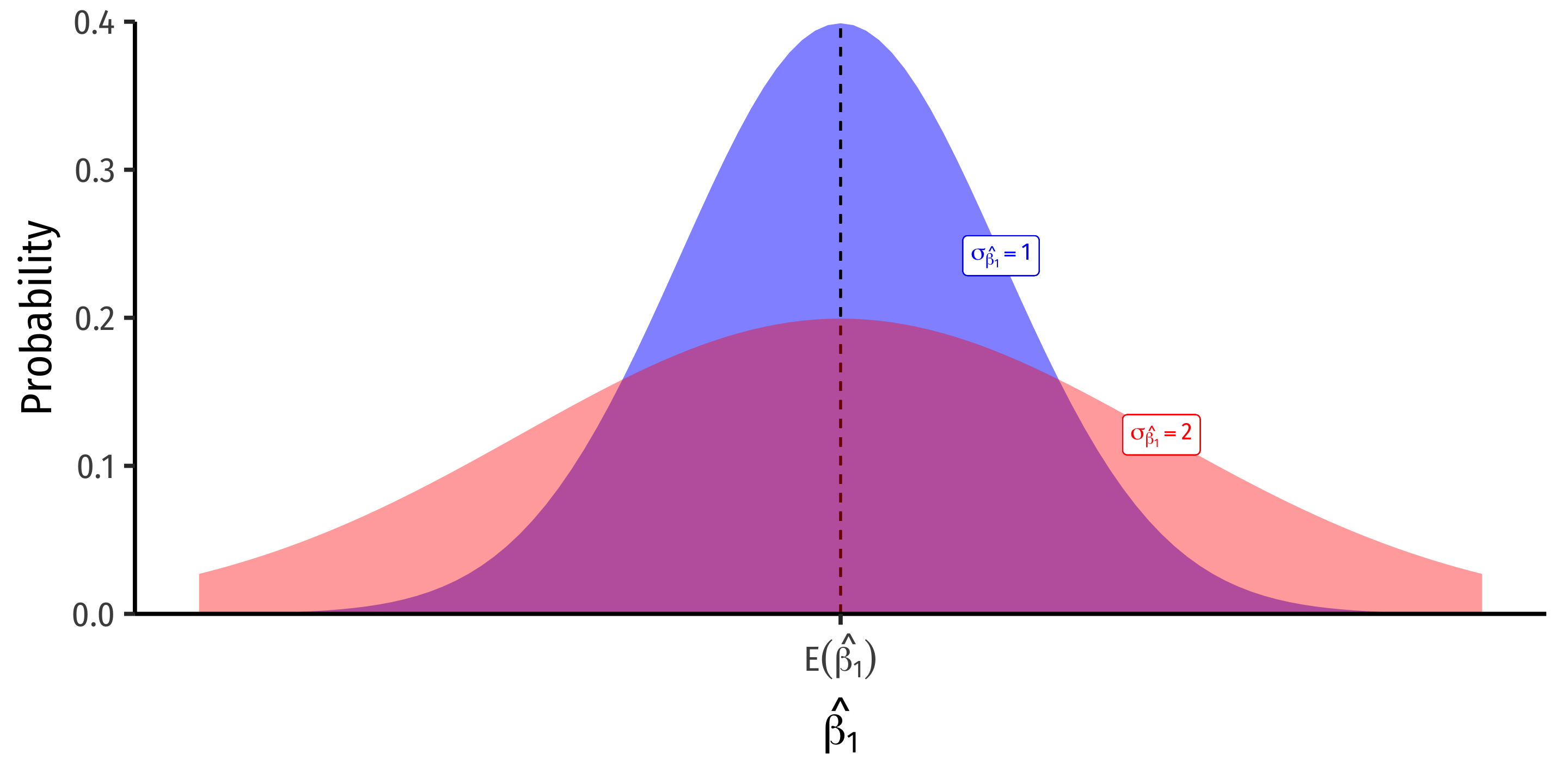
• Precision of OLS estimator ${\hat{\beta }}_1$ measures uncertainty/variability of estimate

  $$\begin{array}{rl}var[{\hat{\beta }}_1]& =\frac{SE{R}^2}{n\times var(X)}\\ se[{\hat{\beta }}_1]& =\sqrt{var[{\hat{\beta }}_1]}\end{array}$$

  • Affected by three factors:

    • Model fit, (SER)

    • Sample size, $n$

    • Variation in $X$

  • Heteroskedasticity & Homoskedasticity

    • Homoskedastic errors (${\hat{u}}_i$) have the same variance over all values of $X$

    • Heteroskedastic errors (${\hat{u}}_i$) have different variance over values of $X$

      • Heteroskedasticity does not bias our estimates, but incorrectly lowers variance & standard errors (inflating $t$-statistics and significance!)

      • Can correct for heteroskedasticity by using robust standard errors

Hypothesis Testing of ${\beta }_1$

• $H_0:{\beta }_1={\beta }_{1,0}$, often $H_0:{\beta }_1=0$

• Two sided alternative $H_1:{\beta }_1\ne 0$

• One sided alternatives $H_1:{\beta }_1>0$ or $H_2:{\beta }_1<0$

• $t$-statistic

$$t=\frac{\widehat{{\beta }_1}-{\beta }_{1,0}}{se(\widehat{{\beta }_1})}$$

• Compare $t$ against critical value $t$*, or compute $p$-value as usual

• Confidence intervals (95%): $\widehat{{\beta }_1}\pm 1.96(se(\widehat{{\beta }_1}))$