
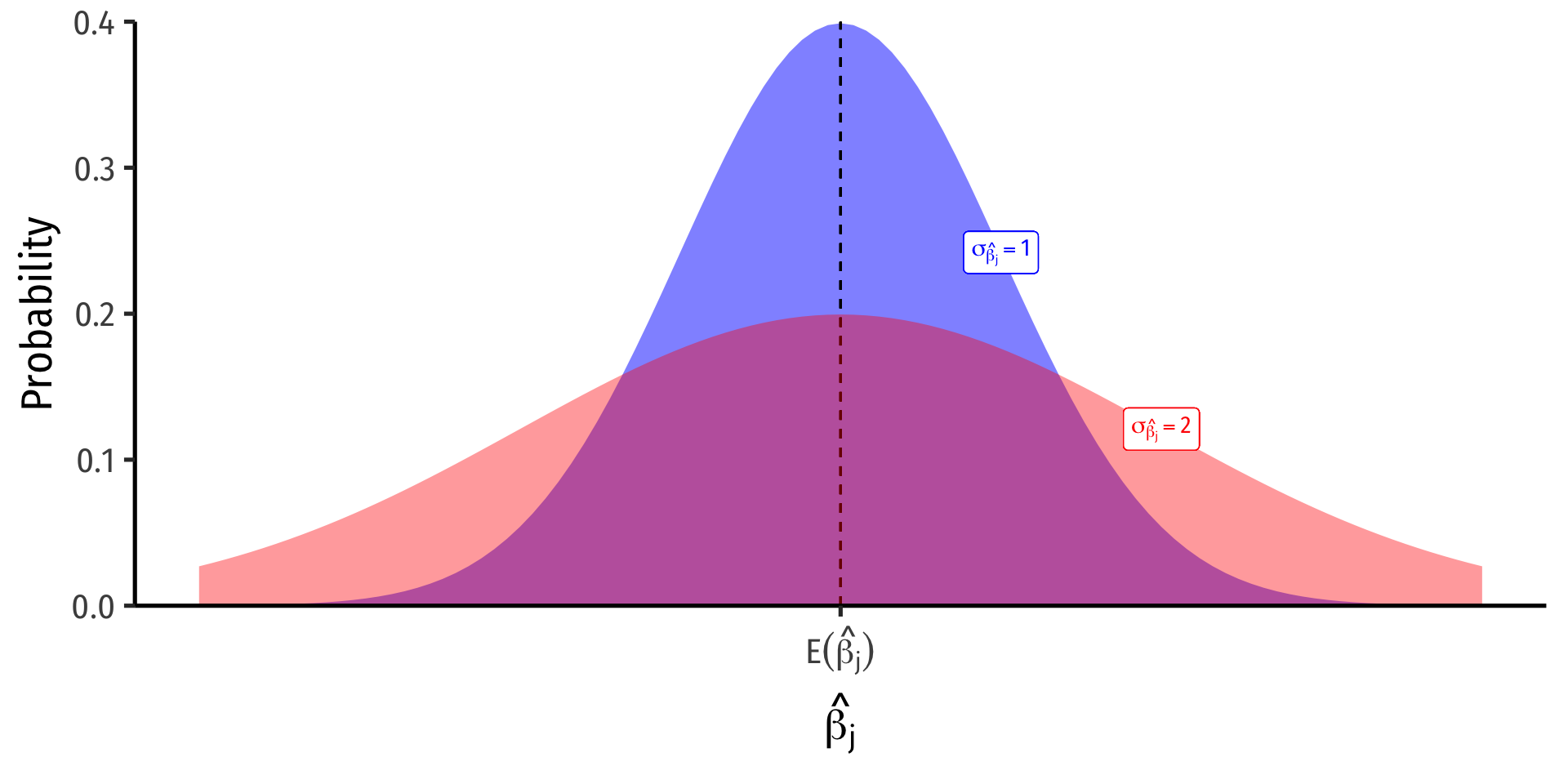
The Sampling Distribution of \(\hat{\beta_j}\)
- For any individual \(\beta_j\), it has a sampling distribution:
\[\hat{\beta_j} \sim N \left(E[\hat{\beta_j}], \;se(\hat{\beta_j})\right)\]
- We want to know its sampling distribution’s:
- Center: \(\color{#6A5ACD}{E[\hat{\beta_j}]}\); what is the expected value of our estimator?
- Spread: \(\color{#6A5ACD}{se(\hat{\beta_j})}\); how precise or uncertain is our estimator?
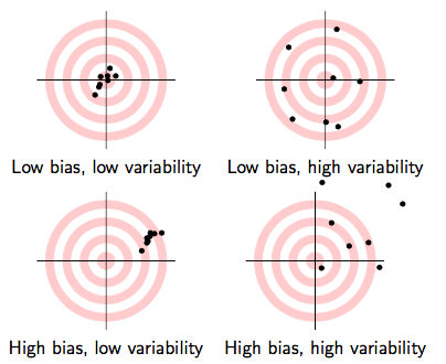
Precision of \(\hat{\beta_j}\) I
\(\sigma_{\hat{\beta_j}}\); how precise or uncertain are our estimates?
Variance \(\sigma^2_{\hat{\beta_j}}\) or standard error \(\sigma_{\hat{\beta_j}}\)
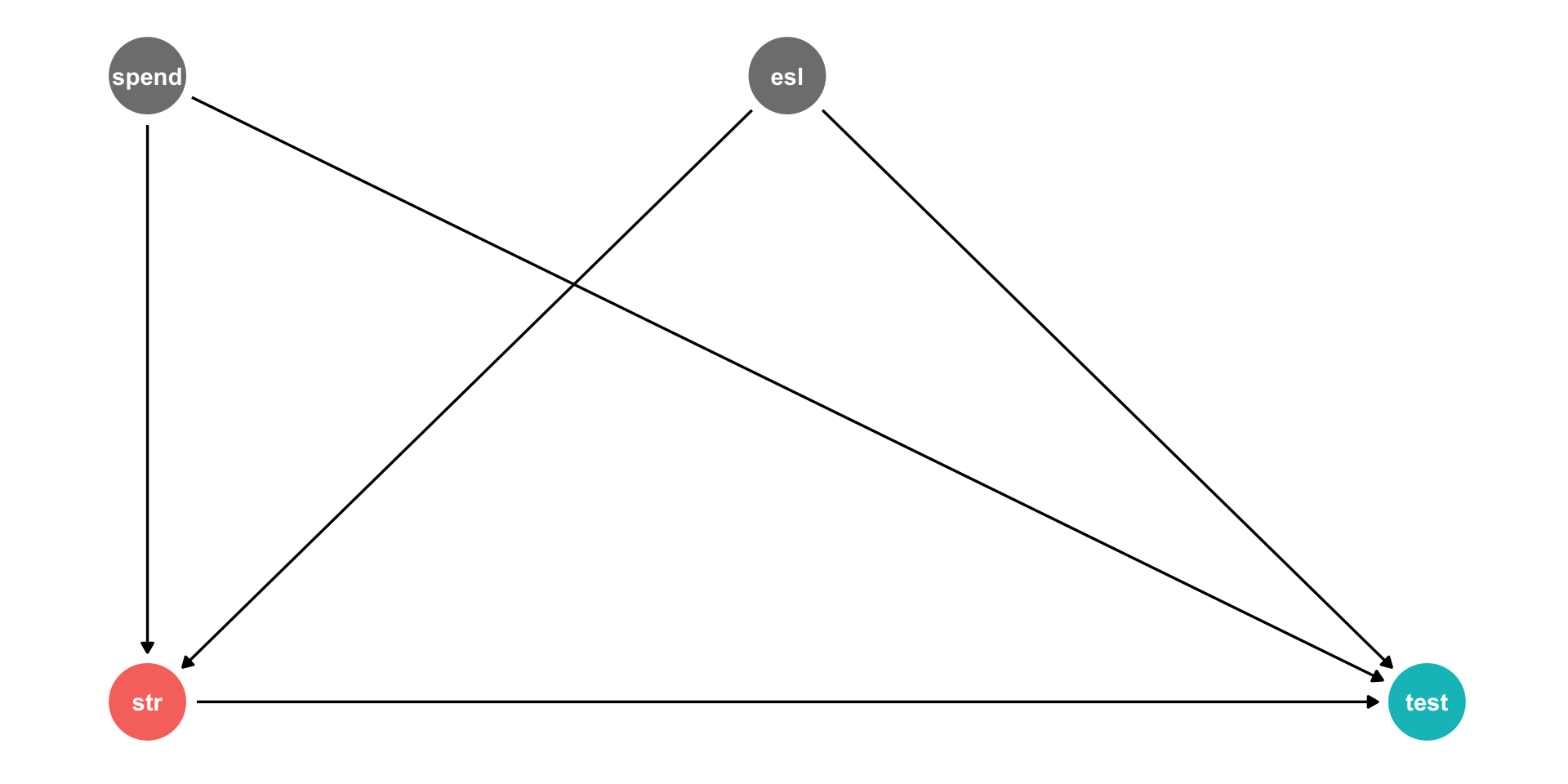
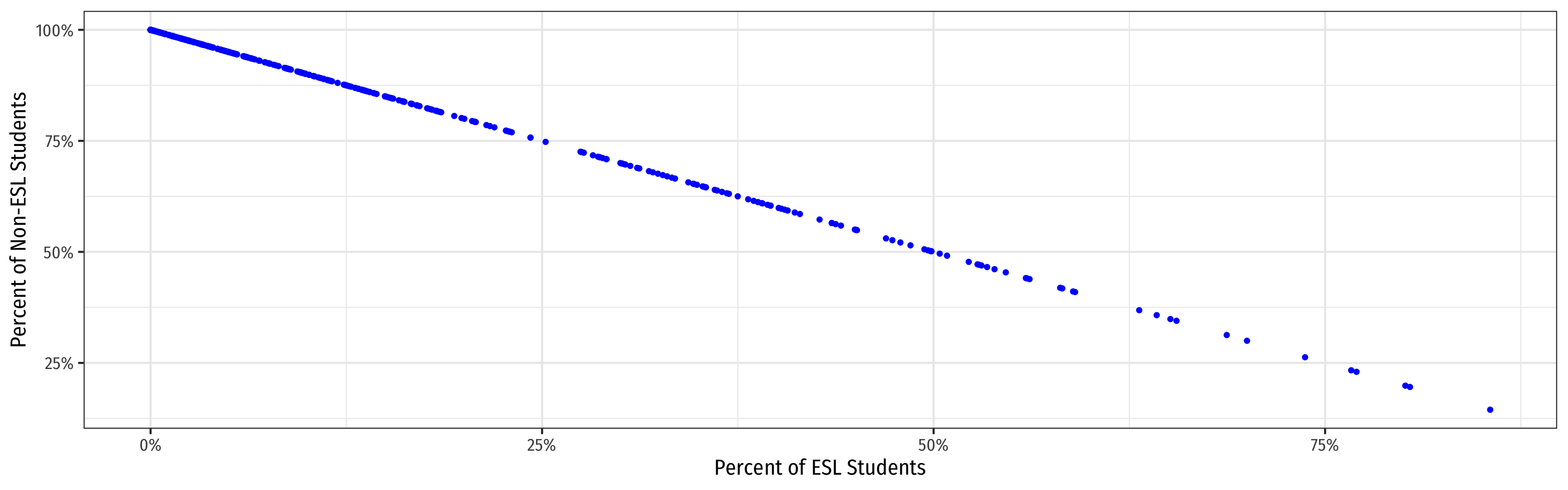
VIF and Multicollinearity in Our Example I
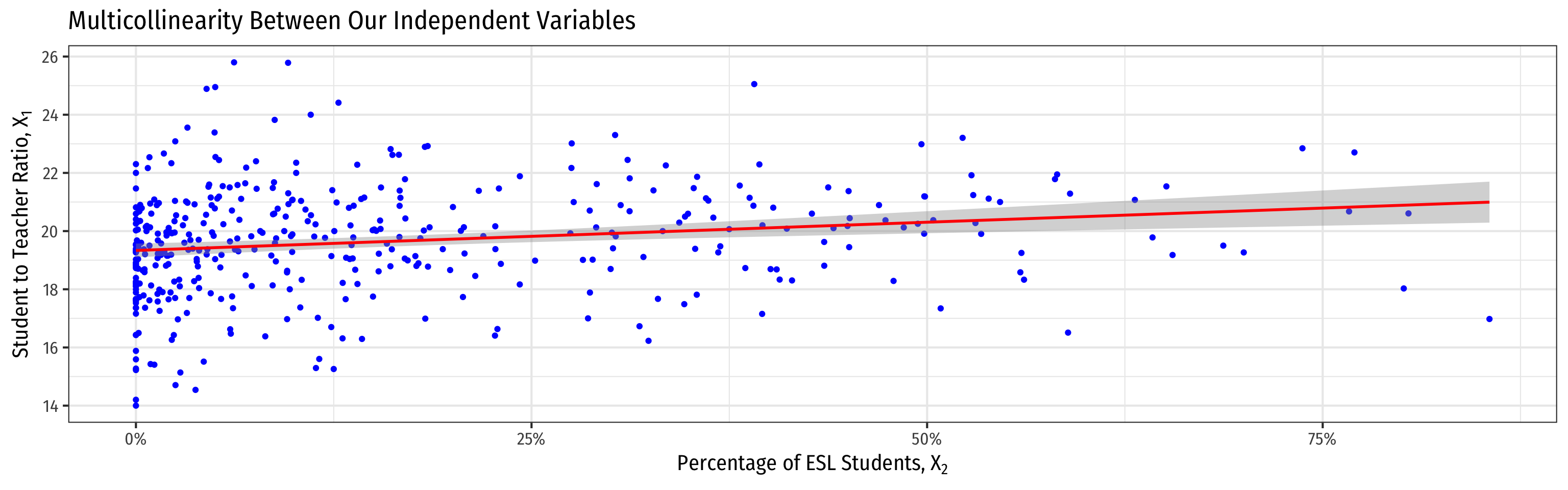
- Higher \(\%EL\) predicts higher \(STR\)
- Hard to get a precise marginal effect of \(STR\) holding \(\%EL\) constant
- Don’t have much data on districts with low STR and high \(\%EL\) (and vice versa)!
Another Example: Expenditures/Student II
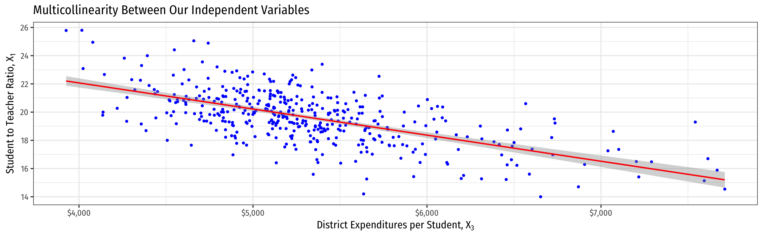
- Higher \(spend\) predicts lower \(STR\)
- Hard to get a precise marginal effect of \(STR\) holding \(spend\) constant
- Don’t have much data on districts with high STR and high \(spend\) (and vice versa)!
Another Example: Expenditures/Student II
Would omitting Expenditures per student cause omitted variable bias?
\(cor(Test, spend) \neq 0\)
\(cor(STR, spend) \neq 0\)
Perfect Multicollinearity: Example III
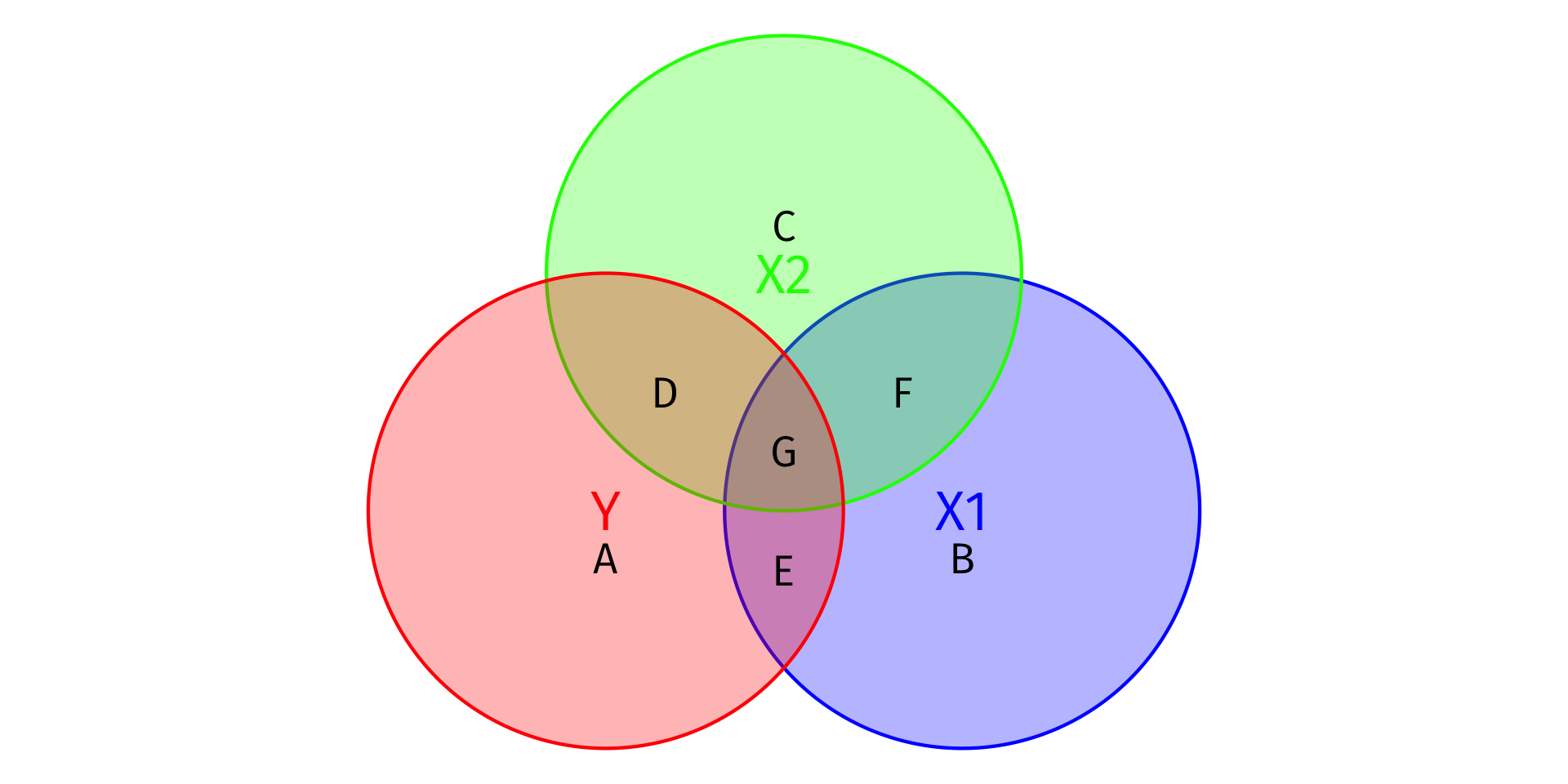
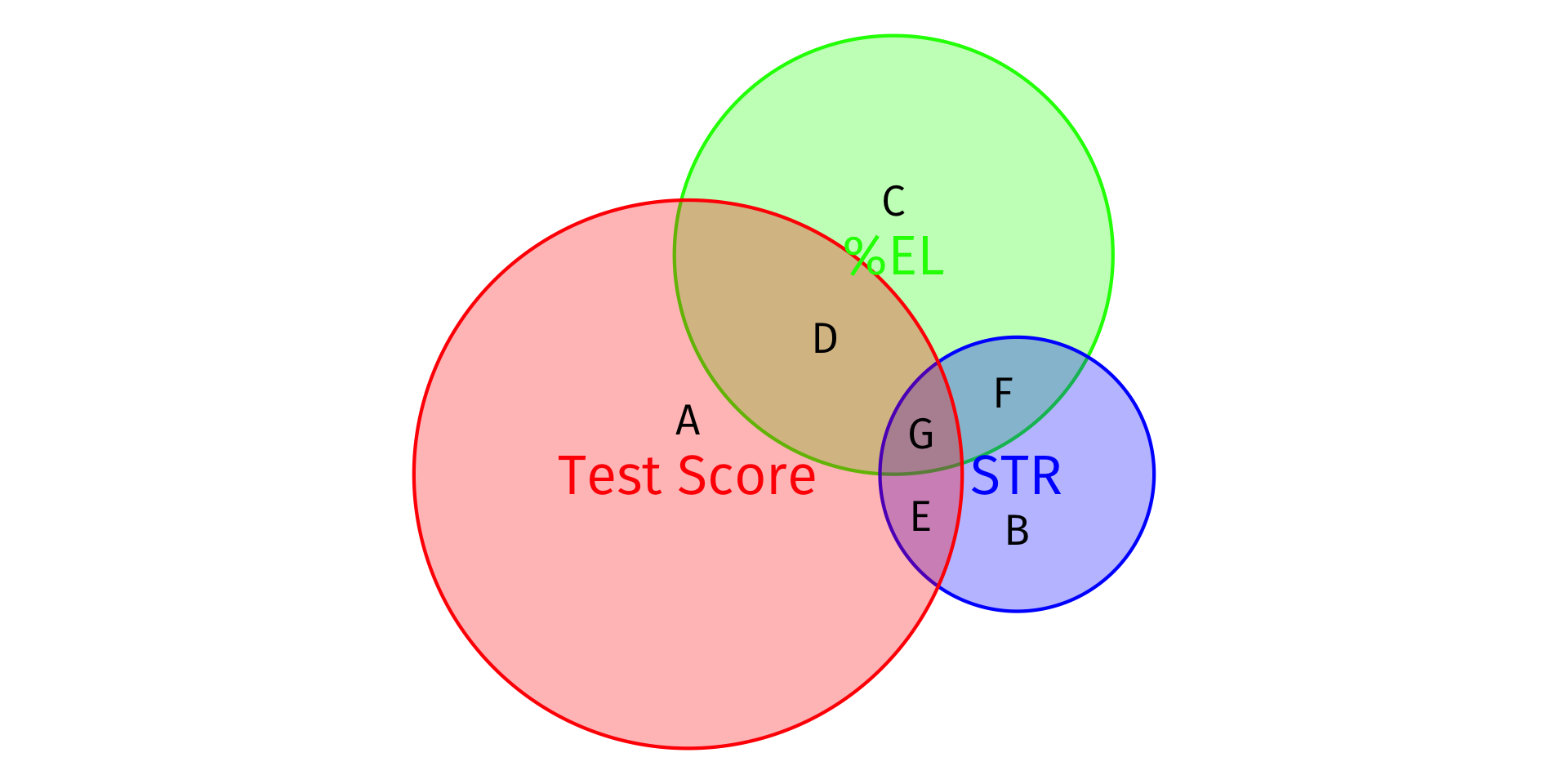
Visualizing \(R^2\)
- Total Variation in Y: Areas A + D + E + G
\[SST = \sum^n_{i=1}(Y_i-\bar{Y})^2\]
- Variation in Y explained by X1 and X2: Areas D + E + G
\[SSM = \sum^n_{i=1}(\hat{Y_i}-\bar{Y})^2\]
- Unexplained variation in Y: Area A
\[SSR = \sum^n_{i=1}(\hat{u_i})^2\]
\[R^2 = \frac{SSM}{SST} = \frac{D+E+G}{\color{red}{A}+D+E+G}\]
Visualizing \(R^2\)
# make a function to calc. sum of sq. devs
sum_sq <- function(x){sum((x - mean(x))^2)}

# find total sum of squares
SST <- elreg %>%
  augment() %>%
  summarize(SST = sum_sq(testscr))

# find explained sum of squares
SSM <- elreg %>%
  augment() %>%
  summarize(SSM = sum_sq(.fitted))

# look at them and divide to get R^2
tribble(
  ~SSM, ~SST, ~R_sq,
  SSM, SST, SSM/SST
  ) %>%
knitr::kable()| SSM | SST | R_sq |
|---|---|---|
| 64864.3 | 152109.6 | 0.4264314 |
\[R^2 = \frac{SSM}{SST} = \frac{D+E+G}{\color{red}{A}+D+E+G}\]
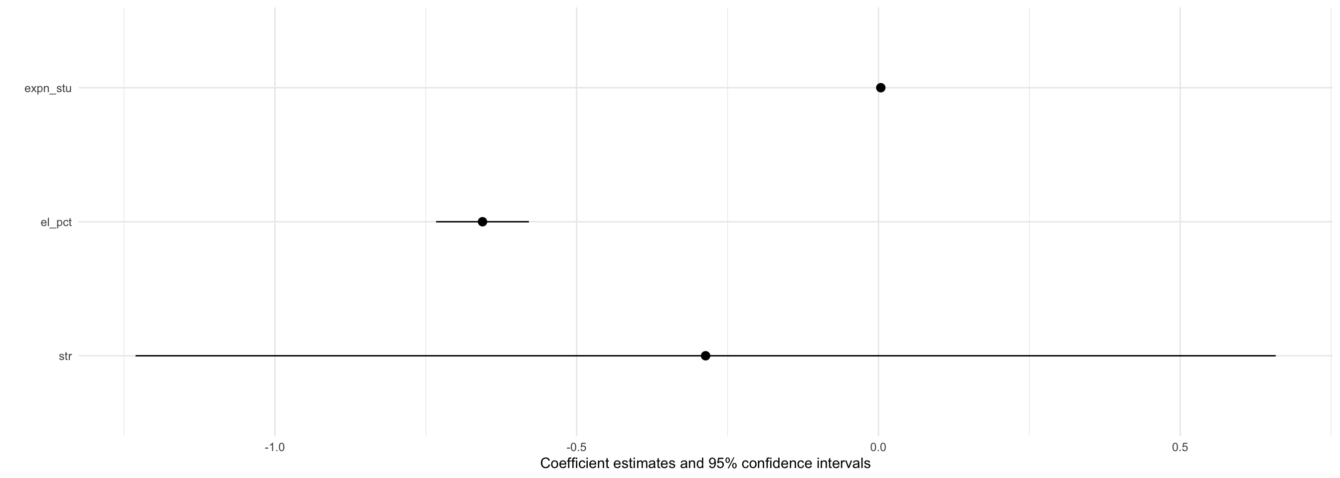
Coefficient Plots (with modelsummary)
Regression Table (with modelsummary)
| Simple Model | MV Model 1 | MV Model 2 | |
|---|---|---|---|
| Constant | 698.93*** | 686.03*** | 649.58*** |
| (9.47) | (7.41) | (15.21) | |
| STR | −2.28*** | −1.10*** | −0.29 |
| (0.48) | (0.38) | (0.48) | |
| % ESL Students | −0.65*** | −0.66*** | |
| (0.04) | (0.04) | ||
| Spending per Student | 0.00*** | ||
| (0.00) | |||
| N | 420 | 420 | 420 |
| Adj. R2 | 0.05 | 0.42 | 0.43 |
| SER | 18.54 | 14.41 | 14.28 |
| * p < 0.1, ** p < 0.05, *** p < 0.01 |
modelsummary(models = list("Simple Model" = school_reg,
                           "MV Model 1" = elreg,
                           "MV Model 2" = reg3),
             fmt = 2, # round to 2 decimals
             output = "html",
             coef_rename = c("(Intercept)" = "Constant",
                             "str" = "STR",
                             "el_pct" = "% ESL Students",
                             "expn_stu" = "Spending per Student"),
             gof_map = list(
               list("raw" = "nobs", "clean" = "N", "fmt" = 0),
               #list("raw" = "r.squared", "clean" = "R<sup>2</sup>", "fmt" = 2),
               list("raw" = "adj.r.squared", "clean" = "Adj. R<sup>2</sup>", "fmt" = 2),
               list("raw" = "rmse", "clean" = "SER", "fmt" = 2)
             ),
             escape = FALSE,
             stars = c('*' = .1, '**' = .05, '***' = 0.01)
)