4.1 — Multivariate OLS Estimators
ECON 480 • Econometrics • Fall 2022
Dr. Ryan Safner
Associate Professor of Economics
safner@hood.edu
ryansafner/metricsF22
metricsF22.classes.ryansafner.com
Contents
The Multivariate OLS Estimators
The Expected Value of ˆβj: Bias
The Multivariate OLS Estimators
The Multivariate OLS Estimators
Yi=β0+β1X1i+β2X2i+⋯+βkXki+ui
- The ordinary least squares (OLS) estimators of the unknown population parameters β0,β1,β2,⋯,βk solves:
min^β0,^β1,^β2,⋯,^βkn∑i=1[Yi−(^β0+^β1X1i+^β2X2i+⋯+^βkXki)⏟ˆYi⏟ˆui]2
- Again, OLS estimators are chosen to minimize the sum of squared residuals (SSR)
- i.e. sum of squared “distances” between actual values of Yi and predicted values ^Yi
The Multivariate OLS Estimators: FYI
Math FYI
in linear algebra terms, a regression model with n observations of k independent variables:
Y=Xβ+u
(y1y2⋮yn)⏟Y(n×1)=(x1,1x1,2⋯x1,nx2,1x2,2⋯x2,n⋮⋮⋱⋮xk,1xk,2⋯xk,n)⏟X(n×k)(β1β2⋮βk)⏟β(k×1)+(u1u2⋮un)⏟u(n×1)
The OLS estimator for β is ˆβ=(X′X)−1X′Y 😱
Appreciate that I am saving you from such sorrow 🤖
The Sampling Distribution of ^βj
- For any individual βj, it has a sampling distribution:
^βj∼N(E[^βj],se(^βj))
- We want to know its sampling distribution’s:
- Center: E[^βj]; what is the expected value of our estimator?
- Spread: se(^βj); how precise or uncertain is our estimator?
The Sampling Distribution of ^βj
- For any individual βj, it has a sampling distribution:
^βj∼N(E[^βj],se(^βj))
- We want to know its sampling distribution’s:
- Center: E[^βj]; what is the expected value of our estimator?
- Spread: se(^βj); how precise or uncertain is our estimator?
The Expected Value of ^βj: Bias
Exogeneity and Unbiasedness
- As before, E[^βj]=βj when Xj is exogenous (i.e. cor(Xj,u)=0)
- We know the true E[^βj]=βj+cor(Xj,u)σuσXj⏟O.V. Bias
- If Xj is endogenous (i.e. cor(Xj,u)≠0), contains omitted variable bias
- Let’s “see” an example of omitted variable bias and quantify it with our example
Measuring Omitted Variable Bias I
- Suppose the true population model of a relationship is:
Yi=β0+β1X1i+β2X2i+ui
- What happens when we run a regression and omit X2i?
- Suppose we estimate the following omitted regression of just Yi on X1i (omitting X2i):1
Yi=α0+α1X1i+νi
Measuring Omitted Variable Bias II
- Key Question: are X1i and X2i correlated?
- Run an auxiliary regression of X2i on X1i to see:1
X2i=δ0+δ1X1i+τi
If δ1=0, then X1i and X2i are not linearly related
If |δ1| is very big, then X1i and X2i are strongly linearly related
Measuring Omitted Variable Bias III
- Now substitute our auxiliary regression between X2i and X1i into the true model:
- We know X2i=δ0+δ1X1i+τi
Yi=β0+β1X1i+β2X2i+ui
Measuring Omitted Variable Bias III
- Now substitute our auxiliary regression between X2i and X1i into the true model:
- We know X2i=δ0+δ1X1i+τi
Yi=β0+β1X1i+β2X2i+uiYi=β0+β1X1i+β2(δ0+δ1X1i+τi)+ui
Measuring Omitted Variable Bias III
- Now substitute our auxiliary regression between X2i and X1i into the true model:
- We know X2i=δ0+δ1X1i+τi
Yi=β0+β1X1i+β2X2i+uiYi=β0+β1X1i+β2(δ0+δ1X1i+τi)+uiYi=(β0+β2δ0)+(β1+β2δ1)X1i+(β2τi+ui)
Measuring Omitted Variable Bias III
- Now substitute our auxiliary regression between X2i and X1i into the true model:
- We know X2i=δ0+δ1X1i+τi
Yi=β0+β1X1i+β2X2i+uiYi=β0+β1X1i+β2(δ0+δ1X1i+τi)+uiYi=(β0+β2δ0⏟α0)+(β1+β2δ1⏟α1)X1i+(β2τi+ui⏟νi)
- Now relabel each of the three terms as the OLS estimates (α’s) and error (νi) from the omitted regression, so we again have:
Yi=α0+α1X1i+νi
- Crucially, this means that our OLS estimate for X1i in the omitted regression is:
α1=β1+β2δ1
Measuring Omitted Variable Bias IV
α1=β1+β2δ1
- The Omitted Regression OLS estimate for X1, (α1) picks up both:
- The true effect of X1 on Y: β1
- The true effect of X2 on Y: β2…as pulled through the relationship between X1 and X2: δ1
- Recall our conditions for omitted variable bias from some variable Zi:
- Zi must be a determinant of Yi ⟹ β2≠0
- Zi must be correlated with Xi ⟹ δ1≠0
- Otherwise, if Zi does not fit these conditions, α1=β1 and the omitted regression is unbiased!
Measuring OVB in Our Class Size Example I
- The “True” Regression (Yi on X1i and X2i)
^Test Scorei=686.03−1.10 STRi−0.65 %ELi
| ABCDEFGHIJ0123456789 |
term <chr> | estimate <dbl> | std.error <dbl> | statistic <dbl> | p.value <dbl> |
|---|---|---|---|---|
| (Intercept) | 686.0322487 | 7.41131248 | 92.565554 | 3.871501e-280 |
| str | -1.1012959 | 0.38027832 | -2.896026 | 3.978056e-03 |
| el_pct | -0.6497768 | 0.03934255 | -16.515879 | 1.657506e-47 |
3 rows
Measuring OVB in Our Class Size Example II
- The “Omitted” Regression (Yi on just X1i)
^Test Scorei=698.93−2.28 STRi
| ABCDEFGHIJ0123456789 |
term <chr> | estimate <dbl> | std.error <dbl> | statistic <dbl> | p.value <dbl> |
|---|---|---|---|---|
| (Intercept) | 698.932952 | 9.4674914 | 73.824514 | 6.569925e-242 |
| str | -2.279808 | 0.4798256 | -4.751327 | 2.783307e-06 |
2 rows
Measuring OVB in Our Class Size Example III
- The “Auxiliary” Regression (X2i on X1i)
^%ELi=−19.85+1.81 STRi
| ABCDEFGHIJ0123456789 |
term <chr> | estimate <dbl> | std.error <dbl> | statistic <dbl> | p.value <dbl> |
|---|---|---|---|---|
| (Intercept) | -19.854055 | 9.1626044 | -2.166857 | 0.0308099863 |
| str | 1.813719 | 0.4643735 | 3.905733 | 0.0001095165 |
2 rows
Measuring OVB in Our Class Size Example IV
“True” Regression
^Test Scorei=686.03−1.10 STRi−0.65 %EL
“Omitted” Regression
^Test Scorei=698.93−2.28 STRi
“Auxiliary” Regression
^%ELi=−19.85+1.81 STRi
- Omitted Regression α1 on STR is -2.28
Measuring OVB in Our Class Size Example IV
“True” Regression
^Test Scorei=686.03−1.10 STRi−0.65 %EL
“Omitted” Regression
^Test Scorei=698.93−2.28 STRi
“Auxiliary” Regression
^%ELi=−19.85+1.81 STRi
- Omitted Regression α1 on STR is -2.28
α1=β1+β2δ1
- The true effect of STR on Test Score: -1.10
Measuring OVB in Our Class Size Example IV
“True” Regression
^Test Scorei=686.03−1.10 STRi−0.65 %EL
“Omitted” Regression
^Test Scorei=698.93−2.28 STRi
“Auxiliary” Regression
^%ELi=−19.85+1.81 STRi
- Omitted Regression α1 on STR is -2.28
α1=β1+β2δ1
The true effect of STR on Test Score: -1.10
The true effect of %EL on Test Score: -0.65
The relationship between STR and %EL: 1.81
So, for the omitted regression:
−2.28=−1.10+(−0.65)(1.81)
Measuring OVB in Our Class Size Example IV
“True” Regression
^Test Scorei=686.03−1.10 STRi−0.65 %EL
“Omitted” Regression
^Test Scorei=698.93−2.28 STRi
“Auxiliary” Regression
^%ELi=−19.85+1.81 STRi
- Omitted Regression α1 on STR is -2.28
α1=β1+β2δ1
The true effect of STR on Test Score: -1.10
The true effect of %EL on Test Score: -0.65
The relationship between STR and %EL: 1.81
So, for the omitted regression:
−2.28=−1.10+(−0.65)(1.81)⏟O.V.Bias=−1.18
Precision of ^βj
Precision of ^βj I
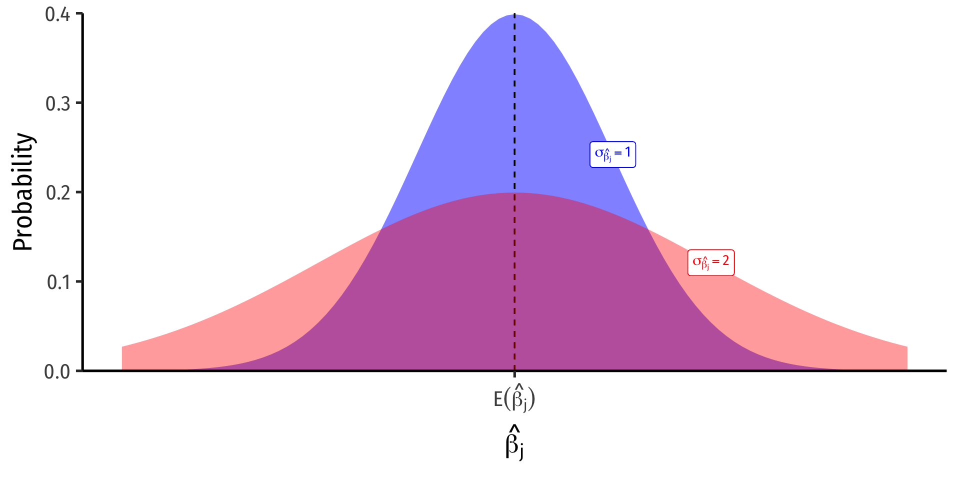
σ^βj; how precise or uncertain are our estimates?
Variance σ2^βj or standard error σ^βj

Precision of ^βj II
var(^βj)=11−R2j⏟VIF×(SER)2n×var(X)
se(^βj)=√var(^βj)
- Variation in ^βj is affected by four things now1:
- Goodness of fit of the model (SER)
- Larger SER → larger var(^βj)
- Sample size, n
- Larger n → smaller var(^βj)
- Variance of X
- Larger var(X) → smaller var(^βj)
- Variance Inflation Factor 1(1−R2j)
- Larger VIF, larger var(^βj)
- This is the only new effect
VIF and Multicollinearity I
- Two independent (X) variables are multicollinear:
cor(Xj,Xl)≠0∀j≠l
- Multicollinearity between X variables does not bias OLS estimates
- Remember, we pulled another variable out of u into the regression
- If it were omitted, then it would cause omitted variable bias!
- Multicollinearity does increase the variance of each OLS estimator by
VIF=1(1−R2j)
VIF and Multicollinearity II
VIF=1(1−R2j)
- R2j is the R2 from an auxiliary regression of Xj on all other regressors (X’s)
- i.e. proportion of var(Xj) explained by other X’s
VIF and Multicollinearity III
Example
Suppose we have a regression with three regressors (k=3):
Yi=β0+β1X1i+β2X2i+β3X3i+ui
- There will be three different R2j’s, one for each regressor:
R21 for X1i=γ+γX2i+γX3iR22 for X2i=ζ0+ζ1X1i+ζ2X3iR23 for X3i=η0+η1X1i+η2X2i
VIF and Multicollinearity IV
VIF=1(1−R2j)
R2j is the R2 from an auxiliary regression of Xj on all other regressors (X’s)
- i.e. proportion of var(Xj) explained by other X’s
The R2j tells us how much other regressors explain regressor Xj
Key Takeaway: If other X variables explain Xj well (high R2J), it will be harder to tell how cleanly Xj→Yi, and so var(^βj) will be higher
VIF and Multicollinearity V
- Common to calculate the Variance Inflation Factor (VIF) for each regressor:
VIF=1(1−R2j)
- VIF quantifies the factor (scalar) by which var(^βj) increases because of multicollinearity
- e.g. VIF of 2, 3, etc. ⟹ variance increases by 2x, 3x, etc.
- Baseline: R2j=0 ⟹ no multicollinearity ⟹VIF=1 (no inflation)
- Larger R2j ⟹ larger VIF
- Rule of thumb: VIF>10 is problematic
VIF and Multicollinearity in Our Example I
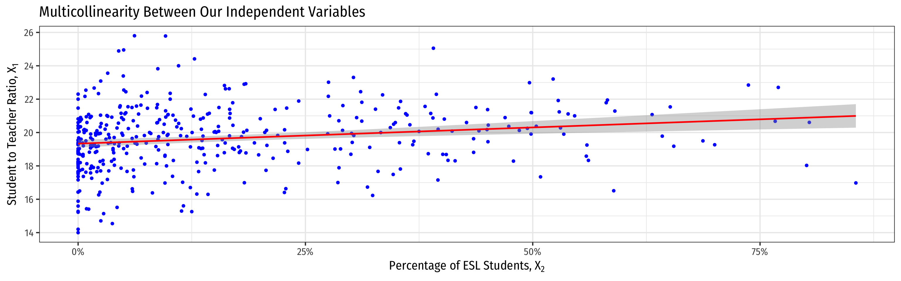
- Higher %EL predicts higher STR
- Hard to get a precise marginal effect of STR holding %EL constant
- Don’t have much data on districts with low STR and high %EL (and vice versa)!
VIF and Multicollinearity in Our Example II
- Again, consider the correlation between the variables
               str    testscr     el_pct
str      1.0000000 -0.2263628  0.1876424
testscr -0.2263628  1.0000000 -0.6441237
el_pct 0.1876424 -0.6441237 1.0000000- cor(STR,%EL)=−0.644
VIF and Multicollinearity in R I
     str   el_pct
1.036495 1.036495 - var(^β1) on
strincreases by 1.036 times (3.6%) due to multicollinearity withel_pct - var(^β2) on
el_pctincreases by 1.036 times (3.6%) due to multicollinearity withstr
VIF and Multicollinearity in R II
- Let’s calculate VIF manually to see where it comes from:
| ABCDEFGHIJ0123456789 |
term <chr> | estimate <dbl> | std.error <dbl> | statistic <dbl> | p.value <dbl> |
|---|---|---|---|---|
| (Intercept) | -19.854055 | 9.1626044 | -2.166857 | 0.0308099863 |
| str | 1.813719 | 0.4643735 | 3.905733 | 0.0001095165 |
2 rows
VIF and Multicollinearity in R III
VIF and Multicollinearity in R IV
[1] 1.036495- Again, multicollinearity between the two X variables inflates the variance on each by 1.036 times
Another Example: Expenditures/Student I
Example
What about district expenditures per student?
Another Example: Expenditures/Student II
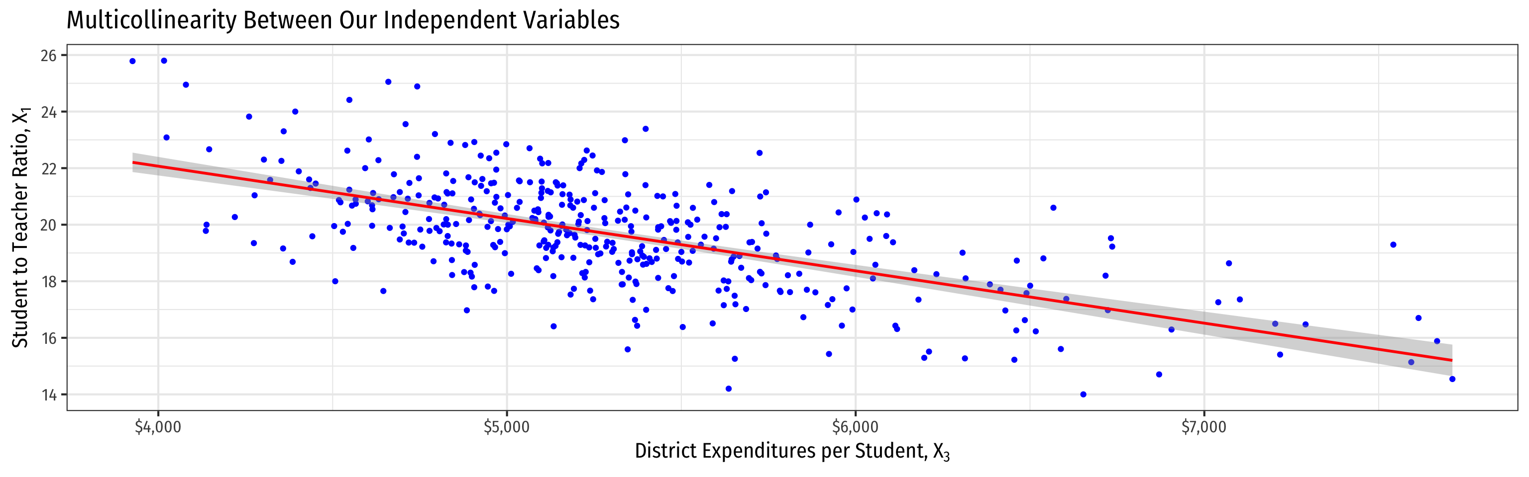
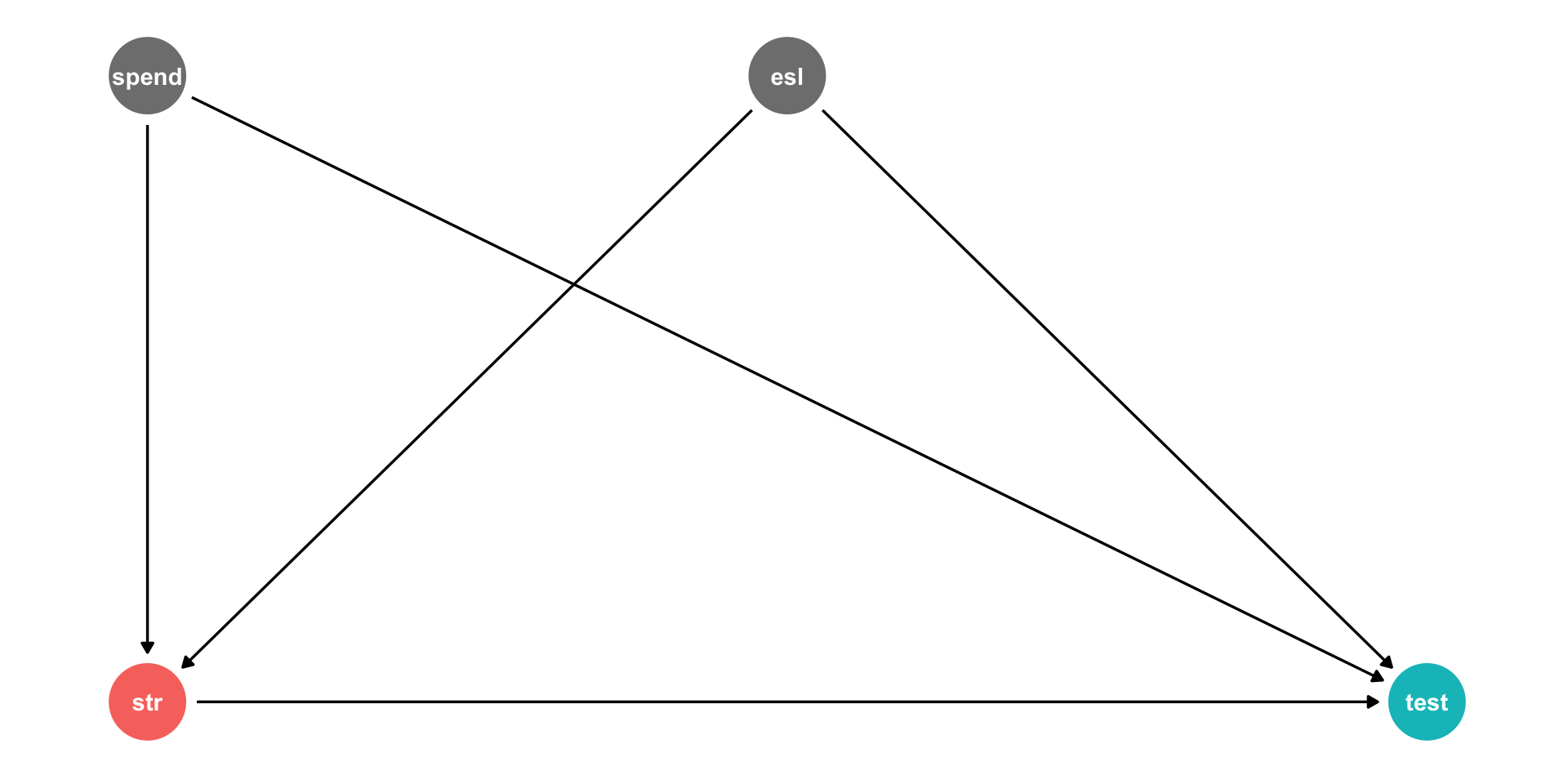
- Higher spend predicts lower STR
- Hard to get a precise marginal effect of STR holding spend constant
- Don’t have much data on districts with high STR and high spend (and vice versa)!
Another Example: Expenditures/Student II
Would omitting Expenditures per student cause omitted variable bias?
cor(Test,spend)≠0
cor(STR,spend)≠0
Another Example: Expenditures/Student III
| ABCDEFGHIJ0123456789 |
term <chr> | estimate <dbl> | std.error <dbl> | statistic <dbl> | p.value <dbl> |
|---|---|---|---|---|
| (Intercept) | 649.577947257 | 15.205718554 | 42.7193194 | 3.299149e-154 |
| str | -0.286399240 | 0.480523198 | -0.5960154 | 5.514891e-01 |
| el_pct | -0.656022660 | 0.039105885 | -16.7755481 | 1.295346e-48 |
| expn_stu | 0.003867902 | 0.001412122 | 2.7390698 | 6.426186e-03 |
4 rows
- Including
expn_stureduces bias but increases variance of β1 by 1.68x (68%)- and variance of β2 by 1.04x (4%)
Multicollinearity Increases Variance
| Test Scores | Test Scores | Test Scores | |
|---|---|---|---|
| Constant | 698.93*** | 686.03*** | 649.58*** |
| (9.47) | (7.41) | (15.21) | |
| Student Teacher Ratio | −2.28*** | −1.10*** | −0.29 |
| (0.48) | (0.38) | (0.48) | |
| Percent ESL Students | −0.65*** | −0.66*** | |
| (0.04) | (0.04) | ||
| Spending per Student | 0.00*** | ||
| (0.00) | |||
| n | 420 | 420 | 420 |
| R2 | 0.05 | 0.43 | 0.44 |
| SER | 18.54 | 14.41 | 14.28 |
| * p < 0.1, ** p < 0.05, *** p < 0.01 |
Perfect Multicollinearity
- Perfect multicollinearity is when a regressor is an exact linear function of (an)other regressor(s)
^Sales=^β0+^β1Temperature (C)+^β2Temperature (F)
Temperature (F)=32+1.8∗Temperature (C)
- cor(temperature (F), temperature (C))=1
- R2j=1→VIF=11−1→var(^βj)=0!
- This is fatal for a regression
- A logical impossiblity, always caused by human error
Perfect Multicollinearity: Example
Example
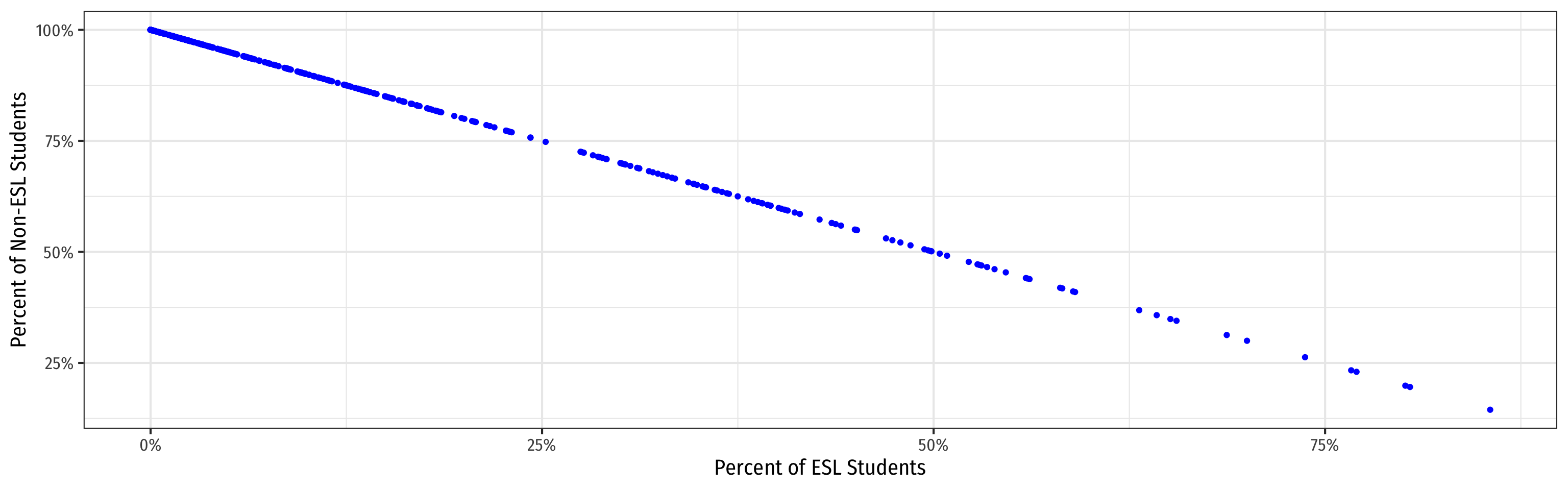
^TestScorei=^β0+^β1STRi+^β2%EL+^β3%EF
%EL: the percentage of students learning English
%EF: the percentage of students fluent in English
%EF=100−%EL
|cor(%EF,%EL)|=1
Perfect Multicollinearity: Example II
| ABCDEFGHIJ0123456789 |
cor <dbl> |
|---|
| -1 |
1 row
Perfect Multicollinearity: Example III
Perfect Multicollinearity Example IV
Call:
lm(formula = testscr ~ str + el_pct + ef_pct, data = ca_school_ex)

Residuals:
    Min      1Q  Median      3Q     Max
-48.845 -10.240  -0.308   9.815  43.461

Coefficients: (1 not defined because of singularities)
             Estimate Std. Error t value Pr(>|t|)
(Intercept) 686.03225    7.41131  92.566  < 2e-16 ***
str          -1.10130    0.38028  -2.896  0.00398 **
el_pct       -0.64978    0.03934 -16.516  < 2e-16 ***
ef_pct             NA         NA      NA       NA
---
Signif. codes:  0 '***' 0.001 '**' 0.01 '*' 0.05 '.' 0.1 ' ' 1

Residual standard error: 14.46 on 417 degrees of freedom
Multiple R-squared:  0.4264,    Adjusted R-squared:  0.4237
F-statistic: 155 on 2 and 417 DF, p-value: < 2.2e-16- Note
Rdrops one of the multicollinear regressors (ef_pct) if you include both 🤡
A Summary of Multivariate OLS Estimator Properties
A Summary of Multivariate OLS Estimator Properties
- ^βj on Xj is biased only if there is an omitted variable (Z) such that:
- cor(Y,Z)≠0
- cor(Xj,Z)≠0
- If Z is included and Xj is collinear with Z, this does not cause a bias
- var[^βj] and se[^βj] measure precision (or uncertainty) of estimate:
var[^βj]=1(1−R2j)∗SER2n×var[Xj]
- VIF from multicollinearity: 1(1−R2j)
- R2j for auxiliary regression of Xj on all other X’s
- mutlicollinearity does not bias ^βj but raises its variance
- perfect multicollinearity if X’s are linear function of others
(Updated) Measures of Fit
(Updated) Measures of Fit
Again, how well does a linear model fit the data?
How much variation in Yi is “explained” by variation in the model (^Yi)?
Yi=^Yi+^ui^ui=Yi−^Yi
(Updated) Measures of Fit: SER
- Again, the Standard errror of the regression (SER) estimates the standard error of u
SER=SSRn−k−1
A measure of the spread of the observations around the regression line (in units of Y), the average “size” of the residual
Only new change: divided by n−k−1 due to use of k+1 degrees of freedom to first estimate β0 and then all of the other β’s for the k number of regressors1
(Updated) Measures of Fit: R2
R2=SSMSST=1−SSRSST=(rX,Y)2
- Again, R2 is fraction of total variation in Yi (“total sum of squares”) that is explained by variation in predicted values (^Yi), i.e. our model (“model sum of squares”)
R2=var(ˆY)var(Y)
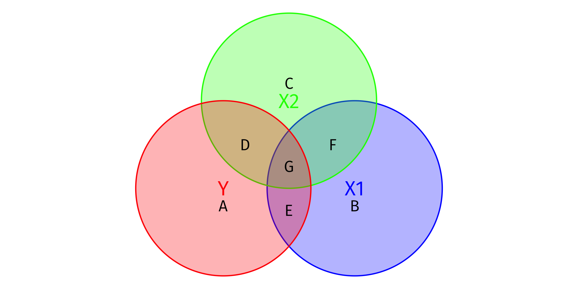
Visualizing R2
- Total Variation in Y: Areas A + D + E + G
SST=n∑i=1(Yi−ˉY)2
- Variation in Y explained by X1 and X2: Areas D + E + G
SSM=n∑i=1(^Yi−ˉY)2
- Unexplained variation in Y: Area A
SSR=n∑i=1(^ui)2
R2=SSMSST=D+E+GA+D+E+G
Visualizing R2
# make a function to calc. sum of sq. devs
sum_sq <- function(x){sum((x - mean(x))^2)}

# find total sum of squares
SST <- elreg %>%
  augment() %>%
  summarize(SST = sum_sq(testscr))

# find explained sum of squares
SSM <- elreg %>%
  augment() %>%
  summarize(SSM = sum_sq(.fitted))

# look at them and divide to get R^2
tribble(
  ~SSM, ~SST, ~R_sq,
  SSM, SST, SSM/SST
  ) %>%
knitr::kable()| SSM | SST | R_sq |
|---|---|---|
| 64864.3 | 152109.6 | 0.4264314 |
R2=SSMSST=D+E+GA+D+E+G
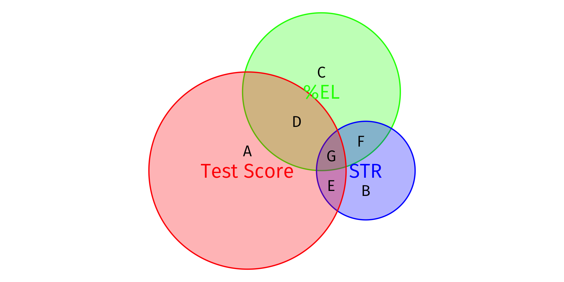
(Updated) Measures of Fit: Adjusted ˉR2
- Problem: R2 mechanically increases every time a new variable is added (it reduces SSR!)
- Think in the diagram: more area of Y covered by more X variables!
- This does not mean adding a variable improves the fit of the model per se, R2 gets inflated
- We correct for this effect with the adjusted ˉR2 which penalizes adding new variables:
ˉR2=1−n−1n−k−1⏟penalty×SSRSST
- In the end, recall R2 was never that useful1, so don’t worry about the formula
- Large sample sizes (n) make R2 and ˉR2 very close
ˉR2 In R
Call:
lm(formula = testscr ~ str + el_pct, data = ca_school)

Residuals:
    Min      1Q  Median      3Q     Max
-48.845 -10.240  -0.308   9.815  43.461

Coefficients:
             Estimate Std. Error t value Pr(>|t|)
(Intercept) 686.03225    7.41131  92.566  < 2e-16 ***
str          -1.10130    0.38028  -2.896  0.00398 **
el_pct       -0.64978    0.03934 -16.516  < 2e-16 ***
---
Signif. codes:  0 '***' 0.001 '**' 0.01 '*' 0.05 '.' 0.1 ' ' 1

Residual standard error: 14.46 on 417 degrees of freedom
Multiple R-squared:  0.4264,    Adjusted R-squared:  0.4237
F-statistic: 155 on 2 and 417 DF, p-value: < 2.2e-16- Base R2 (
Rcalls it “Multiple R-squared”) went up Adjusted R-squared(ˉR2) went down
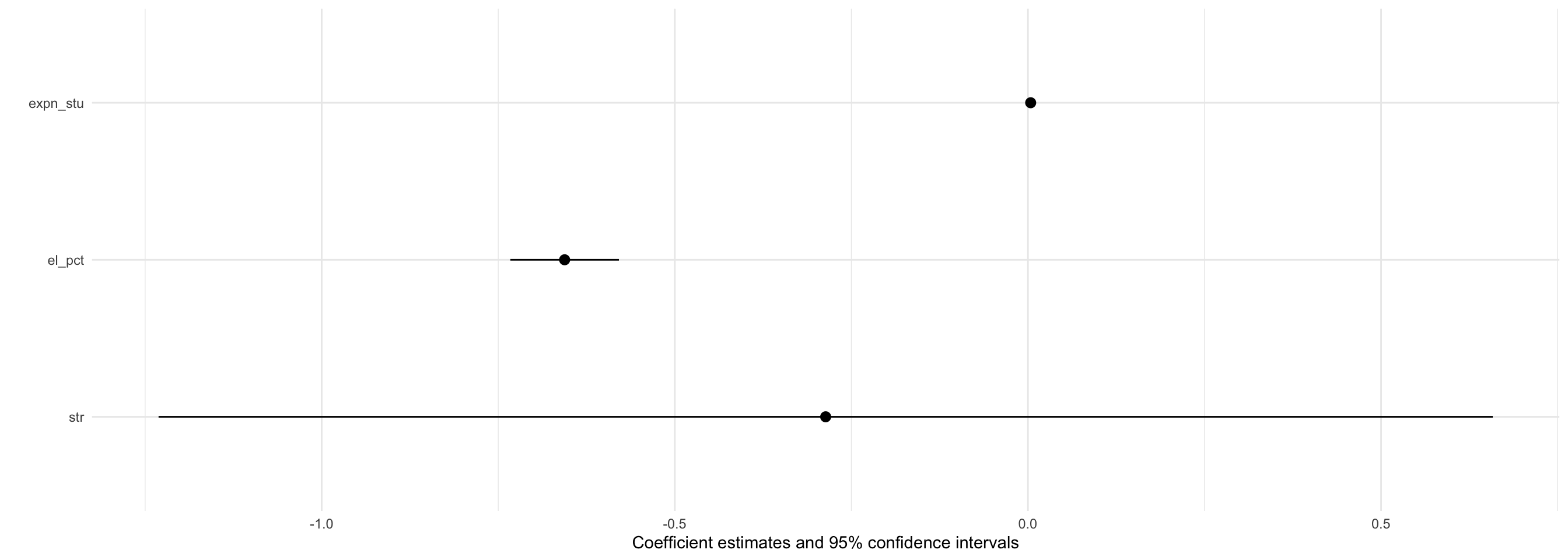
Coefficient Plots (with modelsummary)
Regression Table (with modelsummary)
| Simple Model | MV Model 1 | MV Model 2 | |
|---|---|---|---|
| Constant | 698.93*** | 686.03*** | 649.58*** |
| (9.47) | (7.41) | (15.21) | |
| STR | −2.28*** | −1.10*** | −0.29 |
| (0.48) | (0.38) | (0.48) | |
| % ESL Students | −0.65*** | −0.66*** | |
| (0.04) | (0.04) | ||
| Spending per Student | 0.00*** | ||
| (0.00) | |||
| N | 420 | 420 | 420 |
| Adj. R2 | 0.05 | 0.42 | 0.43 |
| SER | 18.54 | 14.41 | 14.28 |
| * p < 0.1, ** p < 0.05, *** p < 0.01 |
modelsummary(models = list("Simple Model" = school_reg,
                           "MV Model 1" = elreg,
                           "MV Model 2" = reg3),
             fmt = 2, # round to 2 decimals
             output = "html",
             coef_rename = c("(Intercept)" = "Constant",
                             "str" = "STR",
                             "el_pct" = "% ESL Students",
                             "expn_stu" = "Spending per Student"),
             gof_map = list(
               list("raw" = "nobs", "clean" = "N", "fmt" = 0),
               #list("raw" = "r.squared", "clean" = "R<sup>2</sup>", "fmt" = 2),
               list("raw" = "adj.r.squared", "clean" = "Adj. R<sup>2</sup>", "fmt" = 2),
               list("raw" = "rmse", "clean" = "SER", "fmt" = 2)
             ),
             escape = FALSE,
             stars = c('*' = .1, '**' = .05, '***' = 0.01)
)

4.1 — Multivariate OLS Estimators ECON 480 • Econometrics • Fall 2022 Dr. Ryan Safner Associate Professor of Economics safner@hood.edu ryansafner/metricsF22 metricsF22.classes.ryansafner.com